Multi-Scale Turing Patterns

Jonathan McCabe has always created fascinating examples of algorithmic art.

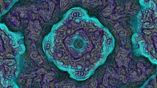
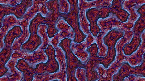
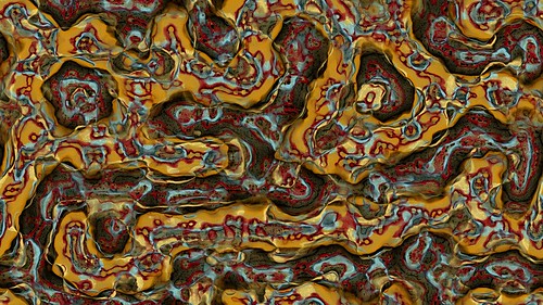
His paper Cyclic Symmetric Mutli-Scale Turing Patterns explains a process that creates very interesting looking images like the following.

With some help from a very patient Jonathan (many thanks Jonathan) he explained the process in more detail so I was able to implement the algorithms myself and experiment.

If you want to play with these patterns they are now included in Visions Of Chaos.

Explanation

Here is my attempted explanation of how the process works – aimed more at the programmer who would like to try implementing it themselves.

The process is based on a series of different turing scales. Each scale has values for activator radius, inhibitor radius, a small amount, weight and symmetry. These are the settings that control the results. For example

Create a main grid 2D array.

Create 3D arrays for activator, inhibitor and variations. In my case I used the format [x,y,scalenum] so each scale has its own dimension within the arrays.

Initialise the grid array to be the size of the image you wish to create and fill it with random floating point values between -1 and +1.

During each step of the simulation;

For each of the mutlitple turing scales;
1. Average each grid cell location over a circular radius specified by activator radius and store the result in the activator array. Multiply by the weight.
2. Average each grid cell location over a circular radius specified by inhibitor radius and store the result in the inhibitor array. Multiply by the weight.
3. Once the averages have been calculated, you need to work out the variation at each grid location. Within a specified variaition radius total up the variation using variation=variation+abs(activator[x,y]-inhibitor[x,y]). Store the variaition for that cell in the variation array. Remember each turing scale needs its own variation array. Smaller variation radii work the best. Checking only a single pixel for the variation formula gives the sharpest most detailed images.

Once you finally have all the activator, inhibitor and variation values for each scale calculated the grid cells can be updated. This is done by;
1. Find which of the scales has the smallest variation value. ie find which scale has the lowest variation[x,y,scalenum] value and call this bestvariation
2. Using the scale with the smallest variation, update the grid value
if activator[x,y,bestvariation]>inhibitor[x,y,bestvariation] then
grid[x,y]:=grid[x,y]+smallamounts[bestvariation]
else
grid[x,y]:=grid[x,y]-smallamounts[bestvariation]

The above step is the main gist of the algorithm. Update a single set of values based on multiple potential scales. That leads to the turing like patterns existing at the different scales within the single image.

Normalise the entire grid values to scale them back to between -1 and +1. ie find the maximum and minimum values across the grid and then update each cell
grid[x,y]:=(grid[x,y]-smallest)/range*2-1;

The grid values can now be mapped to a grayscale value (RGB intensities calculated by trunc((grid[x,y]+1)/2*255)). Alternatively you can map the value into a color palette.

Repeat the process as long as required.

Other Tips

To get images that look like Jonathan’s, you need to have a large difference of activator and inhibitor radius between the different scales. For example

The “Small amount” values really do need to be small. Especially when creating a movie. Otherwise the changes are too rapid and you lose that calm smooth slowly moving effect.

Speedups

After profiling the code, the slowest part of each step is calculating the averaged activator and inhibitor cell values. If using a circular radius then there is a sqrt and two sqr calls to see if the neighbour cell is within the specified radius. The sqrt can be skipped by comparing to the distance squared, but doing this for each scales cells really has an impact on perfromance. Be prepared to wait days if you are generating a movie at even a moderate size. Using the options above rendering a movie at 640×360 for YouTube is taking 27 minutes (!) per frame. All of this time (or 99.9% of it) is spent on the activator and inhibitor averaging, so I needed a much smarter way of doing this.

To help avoid all the distance calculations, you can create a list of neighbour cell offsets before going through each cell. That way when totalling each cells neighbours you use the currecnt cell position minus the saved offset coordinates. This helped speed up the code, but it was still too slow.

Next up was gaussian blur. Gaussian blurring can be simplified to do a pass over the horizontal lines and then the vertical lines of the arrays. This makes it much faster that the large circular averaging method and gave huge speedups (40 seconds per step compared to 27 minutes per step). The results are different to the circular neighbourhood method (as gaussian blurring uses a bell curve weighted kernel for the averaging) but the results are still acceptable.

Then after seeing this page with a fast 2 way rectangular blur I tried that. This gets the time down to 2.2 seconds per step. Using the rectangular neighbourhoods for blur can introduce small scale squared artifacts, but overall the results seem acceptable and the speed increase from 27 minutes per step down to 2.2 seconds per step is very welcome. You can apparently repeat the box blur 3 times to get results that approach a gaussian blur and it is still be faster than the usual gaussian blur. I tried this and it didn’t give the same as the gaussian, but it gets close and leads to more unique results.

Another speedup is related to the symmetries. When implementing the symmetry settings you need to average each of the activator and inhibitor values for each turing scale. This involves a lot of rotation calculations that need sin and cos calcs. It is much faster to precalculate each turing scales symmetry array locations once at the start and then use the precalced list during the main simulation steps. This got the time down to 780 milliseconds per step.

Since this blog post I also refactored the code to be multi-threaded where possible to take advantage of multi-core CPUs. This gives a big jump in performance on modern CPUs.

Result

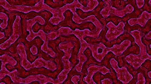
This is the result from using the settings shown above and the fast rectangular blur algorithm to average the activator and inhibitor neighbourhoods.

And here is another sample.

See here for more on multi-scale turing patterns.

Automatically searching for good looking results

Jonathan mentioned histograms in his paper and I have been trying to get my code “smart” enough to detect good or bad sets of random variables.

Each step of the simulation, map the grid cell values into a histogram. X axis is for cell values from -1 to +1. Y axis is the scaled percetage the number of times that cell value occurs.

“Boring” images will have a lot of low histogram counts. The following histogram was just prior to 99% of the values reaching the bottom and leading to a stabilised turing pattern.

The good looking images will have a wider variety of cell values even after many steps. These are the sort of histograms we are interested in detecting.

So once a new set of random variables is set, run the simulation for x number of steps. If most of the histogram values bottom out, then consider it bad and pick another set of variables and start again. If a specified number of steps is reached without a bad histogram, it is potentially good, so save the parameters with a thumbnail image and keep searching. This allows the computer to churn away overnight and look for good images hands free.

The trick is to tweak the bad histogram detection rates to not discard good results while still weeding out the bad results. At this stage I save both the bad and good results into separate folders to make sure it doesn’t discard any good images as bad.

Another method is mutation. Every 1 in 5 (or whatever ratio you like) load one of the good files and mutate the settings slightly. If the mutated image passes the histogram tests then save it with the other good finds.

After trying the histograms method for a while, it doesn’t really work. It will get rid of the most boring results, but between the detected good and bad rules there is no consistancy.

Another method I am trying is to detect how much the main grid array changes between steps. Set totalchange to 0 and then add each grid value totalchange:=totalchange+abs(grid[x,y]-oldgrid[x,y]). After all cells have been tallied you get a changefactor by totalchange/width*height. When auto-searching (after the first 25 steps for settle down) I consider the search bad if the changefactor is >0.01 or <0.006. This helps weed out a few more of the boring results, but there are still too many good results detected as bad and too many bad results detected as good.

So there needs to be smarter ways to try and find the best looking results without all the false-positives.

Adding Color

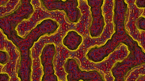
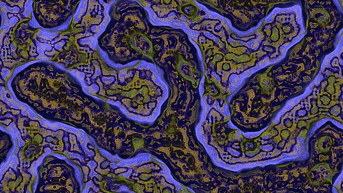
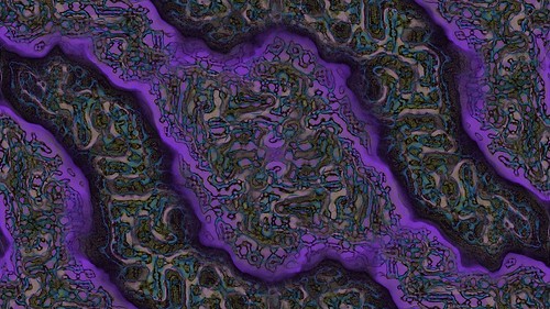
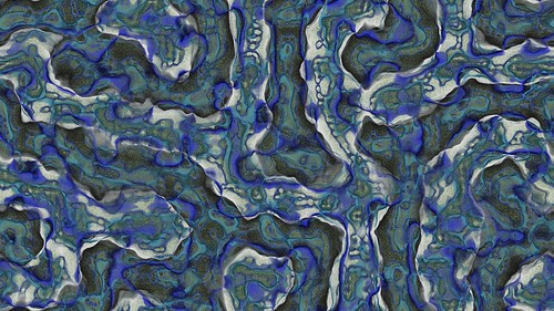
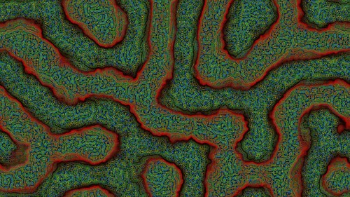
Make sure you click these images to see the full 4K resolution details.

I wanted to add color to the output images for a long time. Various methods I tried were not impressive (mapping the pixel brightness levels to a color palette or converting RGB to HSL all gave disappointing results).

Then I saw Ricky Reusser‘s twitter posts on how he had implemented and extended his Multi-scale Turing Pattern code to output color images. See his blog post here for more info.

To inject color into the Turing patterns the usual steps as described above are used except for a few small changes;

1. Before you start the steps, create a 2D array of colors that is the same size as the display image. Set all the values to the same starting color. I found black is a nice choice as the various colors fade in as the Turing steps run.

2. Set a different color for each of the scales. They can be any color, but brighter colors tend to work best.

3. At the point in the steps you find the bestvariation, you “bump” the current pixel color towards the scale color. For example if the best variation turns out to be the 2nd scale and that scale has a color of red RGB(255,0,0) you move the white color towards red. For the bump/move I used a simple linear interpolation (LERP).

target=trunc((current*(1-bumpamount))+(scalecolor*bumpamount))

This allows the colors to smoothly change as the steps of the simulation run.

4. To display the colors, you multiply the pixel color by the intensity of the grid value (grid[x,y]-1)/2.

That gives you the color shading. Some brightness and contrast tweaks can help bring out the colors a bit more.

This is also another example of the value of shared knowledge. Without this original blog post Ricky may never have seen these Turning patterns. Because of sharing the how to, he was able to come up with a new idea to extend the results further. I encourage everyone to share any knowledge you have to others.

Here is a sample movie of some color results.

More Color Ideas

Blake Jones has other coloring methods for turing patterns he describes here that I really need to experiment with when I get some time.

Jason.