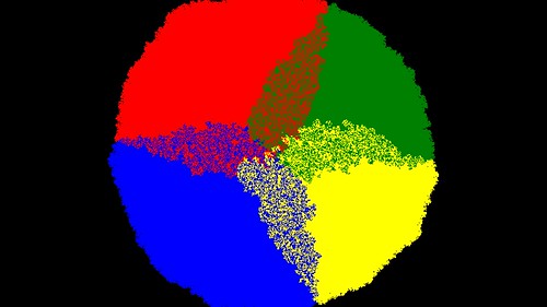
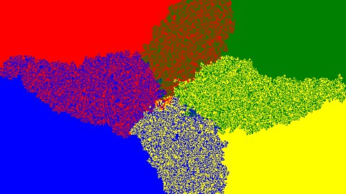
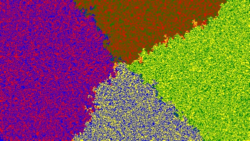
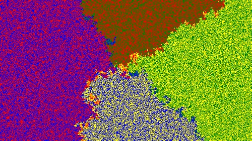
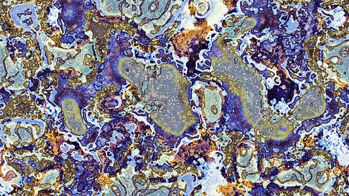
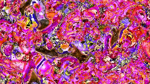
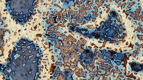
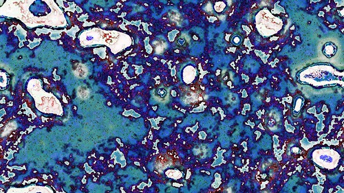
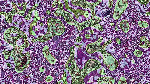
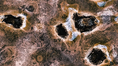
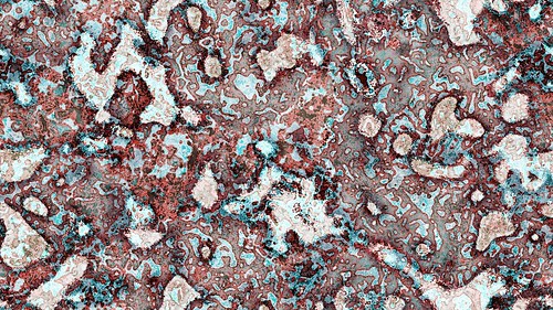
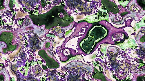
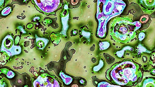
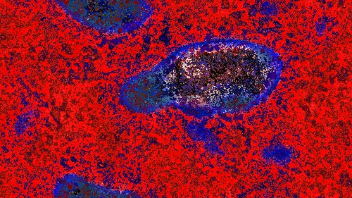
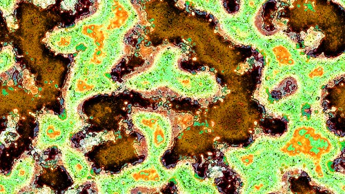
Make sure you click the images in this post to see them in full 4K resolution. The thumbnails do not do them justice and hide a lot of the multi-scaled structures within them.

After my original attempt to replicate Jonathan McCabe‘s Coupled Cellular Automata results I was contacted by Ian McDonald with some questions about how my original algorithms worked and that inspired both of us to make another attempt at getting McCabe like results.

With some back and forth and some hints from Jonathan we were able to get a little further towards replicating his images.

How the McCabe algorithms work
Jonathan has provided some hints to how his Coupled CA work in the past.
Firstly from here;
Each pixel represents the state of the 4 cells of 4 cellular automata, which are cross coupled and have their individual state transition tables. There is a “history” or “memory” of the previous states which is used as an offset into the state transition tables, resulting in update rules which depend on what has happened at that pixel in previous generations. Different regions end up in a particular state or cycle of states, and act very much like immiscible liquids with surface tension.

and secondly from here;
The generative system involves four linked cellular automata – think of them as layers. “Linked” because at each time step, a cell’s state depends both on its neighbours in that layer, and on the states of the corresponding cells in the other three layers. Something like a three-dimensional CA, but not quite; the four layers influence each other through a weighted network of sixteen connections (a bit like a neural net). The pixels in the output image use three of the four CA layers for their red, green and blue values.
As in a conventional CA, each cell looks to its neighbours to determine its future state. This is a “totalistic” CA, which means each simply sums the values of its neighbours, then changes its state based on a table of transition rules. Now for the really good part: each cell also uses its recent history as an “offset” into that transition table. In other words, the past states of a cell transform the rules that cell is using. The result is a riot of feedback cycles operating between state sequences and rulesets; stable or periodically oscillating regions form, bounded by membrane-like surfaces where these feedback cycles compete. Structures even form inside the membranes – rule/state networks that can only exist between other zones.

After emailing him he did provide a few more more clues to how his Coupled CA work which did help me get to the point I am at now.
How the “inner loop” behaves and how the 4 (or more) CA layers are actually processed and combined is still a mystery, but this is a hint;
“Cross-Coupled” is a matrix multiply to give 4 numbers from 4 numbers. If the matrix was “1.0” diagnally and “0.0” elsewhere you have zero coupling. If the zeros are replaced with other values you get cross-coupling of various amounts. If the cross coupling is very low you have 4 independant systems, if it is very high you get effectively one system, I think there is a sweet spot in between where they influence each other but don’t disappear into the mix.
And regarding the history;
The history or memory is an average of previous states at that cell. You can do it a few ways, say as a decaying average, adding the current state and multiplying by 0.99 or some number, so the memory fades. The memory is added to the index to look up the table, so you actually need a bigger table than 9*256.

How my version works
Here are the basic steps to how I created the images within this post. Note that this is not how the McCabe CA works, but does show some similarities visually to his.
The CA is based on a series of CA layers. Each layer/array constains byte values (0-255) and is initialised with random noise. You need a minimum of 4 layers, but any number of layers can be used.
You also need a set of lookup tables for each layer. The lookup tables are 1D arrays containing byte values (0-255). They each have 256*10 entries. The arrays are filled using multiple sine waves combining different frequencies and amplitudes which are then normalised into the 0-255 range. You want to have smallish changes between the lookup table entries.
256*10 entries in the lookup table is because in the McCabe CA the current cell, its 8 neighbours and the history of that cell are used to index the lookup table. That gives 10 possible values between 0 and 255 which are totalled to index the lookup table. For the method I discuss in this blog post, you really only need a lookup table with 256 entries as the index maths never goes betyond 0 to 255. BUT I still use the larger sized array to stretch the sine waves further/more smoothly across the tables. Note you can also change the “*10” size to a larger number to help smooth out the resulting CA displays even more. Experiment with different values.

Now for the main loop.
1. Blur each layer array. Gaussian blur can be used but tends to be slow. Using a faster 2 pass blur as described here works just as well for this purpose. Make sure the blur radius has a decent amount of difference between layers, for example 1, 10, 50, 100. These large differences in blur amounts is what leads to the resulting images having their detail at many scales appearance.

2. Process the layers. This is the secret step that Jonathan has not yet released. I tried all sorts of random combinations and equations until I found the following. This is what I use in the images for this post.
for i:=0 to numlayers-1 do t[i,x,y]:=c[i,x,y]+lookuptable[i,trunc(abs(h[(i+1) mod numlayers,x,y]-c[(i+2) mod numlayers,x,y]))];
That allows for any number of layers, but to show the combinations simpler, here it is unrolled for 4 layers
t[0,x,y]:=c[0,x,y]+lookuptable[0,trunc(abs(h[1,x,y]-c[2,x,y]))];
t[1,x,y]:=c[1,x,y]+lookuptable[1,trunc(abs(h[2,x,y]-c[3,x,y]))];
t[2,x,y]:=c[2,x,y]+lookuptable[2,trunc(abs(h[3,x,y]-c[0,x,y]))];
t[3,x,y]:=c[3,x,y]+lookuptable[3,trunc(abs(h[0,x,y]-c[1,x,y]))];
t is a temp array. Like all CAs you put the results into a temp array until the whole grid is processed and then you copy t back to c
c is the current CA layers array
lookuptable is the array created earlier with the combined sine waves
h is the history array, ie what the c array was last cycle/step
An important step here is to blur the arrays again once they have been processed. Using just a radius 1 gaussian is enough. This helps cut down the noise and speckled nature of the output.
To make it a little more clear here is the main loop code that does the processing of the arrays.
//blur each layer
for i:=0 to numlayers-1 do QuickBlurArray(c,i,strtoint(CoupledCA2Options.grid.Cells[1,i+1]));

//process the layers
for y:=0 to imageheight-1 do
begin
     for x:=0 to imagewidth-1 do
     begin
          for i:=0 to numlayers-1 do t[i,x,y]:=c[i,x,y]+lookuptable[i,trunc(abs(h[(i+1) mod numlayers,x,y]-c[(i+2) mod numlayers,x,y]))];
     end;
end;

//update main arrays from temp arrays
for y:=0 to imageheight-1 do
	for x:=0 to imagewidth-1 do
		for i:=0 to numlayers-1 do
			c[i,x,y]:=t[i,x,y];

//quick blur each of the CA layers
for i:=0 to numlayers-1 do QuickBlurArray(c,i,1);

//save current state into history array
for y:=0 to imageheight-1 do
    for x:=0 to imagewidth-1 do
        for i:=0 to numlayers-1 do
            h[i,x,y]:=c[i,x,y];
Hope that helps clarify.

3. Display. So now you have 4 byte vlaues (one for each layer) for each pixel. How can you convert these into a color to display? So far I have used these methods;
Color palette – Average the 4 values and use them as an index into a 256 color palette.
RGB – Use the first 3 layers as RGB components.
YUV – Use the first 3 layers as YUV components and then convert into RGB.
Matrix coloring – This deserves a larger section below.

Matrix coloring
If you use just RGB or YUV conversions the colors tend to be a bit bland and unexciting. When I asked Jonathan how he got the amazing colors in his images he explained that the layers can be multiplied by a matrix. Now, in the past I had never really needed to use matrices except in some OpenGL code (and even then OpenGL handles most of it for you) but a quick read of some online tutorials and I was good to go.
You take the current cell values for 3 layers and multiply them by a 3×3 matrix
              [m2 m2 m2]
[m1 m1 m1]  x [m2 m2 m2] = [m3 m3 m3]
              [m2 m2 m2]
or 4 layers multiplied by a 4×4 matrix
                 [m2 m2 m2 m2]
                 [m2 m2 m2 m2]
[m1 m1 m1 m1]  x [m2 m2 m2 m2] = [m3 m3 m3 m3]
                 [m2 m2 m2 m2]
In both cases the m1 array variables are the CA layer values for each of the X and Y pixel locations. I use the first 3 layers, last 3 layers or first layer and last 2 layers. If you use a 4×4 matrix use the first 4 etc. Multiply them by the m2 matrix and get the m3 results.
You can use the m3 results as RGB components to color the pixels (after multiplication the RGB values will be outside the normal 0 to 255 range so they will need to be normalised/scaled back into the 0 to 255 range). For the 4×4 matrix you can use the 4th returned value for something too. I use it for a contrast setting but it doesn’t make that much of a difference.
If the matrix you are multiplying is the identity matrix (ie all 0s with diagonal 1s) the m3 result is the same as the m1 input. If you change the 0s slightly you get a slight change. For the images in this post I have used random matrix values anywhere from -10 to +10 (with and without a forced diagonal of 1s).
Using matrix multiplication to get the wider range of colors is really awesome. I had never seen this method used before and am so grateful of the hint from Jonathan. I am sure it will come in handy in many other areas when I need to convert a set of values to colors.
Another great tip from Jonathan is to do histogram equalisation on the bitmap before display. This acts like an auto-contrast in Photoshop and can really make blander images pop.
Another thing to try is hue shifting the image. Convert each pixel’s RGB values to HSL, shift the H component and then convert back to RGB.

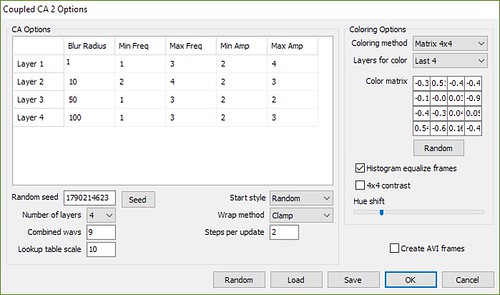
Once you put all those options together you get might get a dialog with a bunch of settings that looks like the following screen shot.

Problem
There is one major issue with this method though. You cannot create a nice smooth evolving animation this way. The cell values fluctuate way too much between steps causing the movie to flicker wildly. To help reduce flicker you can render only every second frame, but the movie still has wild areas. Jonathtan confirmed his method also has the same display results. Coupled Cellular Automata using the method described in this post are best used for single frame images and not movies.

Help me
If you are a fellow cellular automata enthuisast and have a play with this method, let me know of any advancements you make. Specifically, the main area that can be tweaked is the inner loop algorithm of how the layers are combined and processed. I am really interested in any variations that people come up with.

Explore it yourself
If you are not a coder and want to experiment with Coupled Cellular Automata they are now included in Visions of Chaos.
To see my complete gallery of Coupled Cellular Automata images click here.
Jason.
