Mitchell Gravity Set Fractals

Origins

Back in the 1980’s Fred Mitchell designed a method to visualize Newtonian gravity he called the Mitchell Gravity Set or MGS. See here for his page explaining MGS.

This process of plotting dynamic systems is usually referred to as basins of attraction. See this paper and this paper for other versions of plotting gravitational basins of attraction. Similar methods are used when plotting Root-Finding Fractals and the basins of a Magnetic Pendulum.

The 2D images in this post are from when I first experimented with MGS back in 2005.

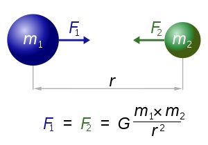
The basics of MGS is that you have a number of gravity objects (stars or gravity wells) in 2D space. Each pixel of a 2D image becomes the starting coordinate for a particle in that 2D space. The particle is attracted to the stars through Newtonian gravity and moves. You follow the path the particle takes for a number of steps and color the pixel depending on how long it took to be flung out of the simulation area.

I ended up rewriting/translating my old code into GLSL for speed. Click here to see the shader source code that generates these 2D Gravity Set images.

By playing with the various star positions and masses you can get a variety of different images.

The following image shows the current Gravity Set Options dialog in Visions of Chaos showing the various settings that can be tweaked.

Revisiting and Extending Into The 3rd Dimension

I was recently contacted by Fred again and he mentioned he was working on getting a 3D version of MGS going. Getting the 2D code going in 3D is simple enough. Just a few extra lines for adding the Z dimension, so I was inspired to have a go at seeing what the 3D versions could look like. The settings dialog is extended as follows.

Similar to the other 3D grid based displays like 3D Cellular Automata I have worked with, displaying a 3D grid of values can be tricky.

The following examples use a 500x500x500 resolution space.

The most obvious is a 3D Grid of little cubes. Each smaller cube is a starting point for the gravity calculations. Color the cubes depending on which gravity well they come closest to during their journey.

That gives you a general idea of what the shapes of the 3D Gravity Set will be, but the interior is completely hidden.

You can slice an eighth of the cubes away….

or even slice a half…

Another option is to only display the cubes for only half of the gravity wells….

or even for only a single well.

Then came the idea for “volumetric rendering”. I already had code for rendering transparent billboard quads so I used that. I am only rendering the edges of each gravity well area. If you render all points the image is just a white blob mess.

Another method. Export the visible cubes as a OBJ point cloud. Import the OBJ into MeshLab. Use MeshLab to generate normals for the points and then marching cubes to generate a mesh from the point cloud. Export the mesh as a PLY format file. Import the PLY into Blender and render it. These are rough results. I am sure someone who knows more about MeshLab and Blender could clean up the mesh and make a much better looking render.

Here is a sample movie of rotating gravity sets.

Magnetic Pendulum Alternative to MGS

I also tried using Magnetic Pendulum formulas in 3D to do similar plots. The formula is a 3D extension of the 2D code I used here. Otherwise the rest of the code is the same as for the 3D MGS above.

Availability

Both 2D and 3D Gravity Set Fractals are now included in the latest version of Visions of Chaos.

Jason.

More adventures with 3D Gravity simulations and OpenCL

History

3D Gravity simulations are something I have been interested in for many years now. Some worked, some didn’t, some were more realistic than others.

The first 3D Gravity simulation movie I still have on my YouTube channel is this one from way back in May of 2007. Low res with only a bunch of blurry objects.

Since then I have increased the details and object counts. I also started experimenting with OpenCL for big speedups that allowed many more objects to be simulated in a reasonable time frame.

Moving forward to now

For this latest post I went back and rewrote my code and the OpenCL kernel code to correctly compare every object to all other objects in the gravity calculations. The simulation is using Newton’s law of universal gravitation.

Every point mass attracts every single other point mass by a force acting along the line intersecting both points. The force is proportional to the product of the two masses and inversely proportional to the square of the distance between them.

How this simulation works

I am using software OpenGL on the CPU for all the rendering of the visuals and CPU and OpenCL for the gravity calculations. OpenCL code runs on your graphics card GPU and GPUs are great at running lots of small bits of code fast at the same time. The gravity formula maths is perfect for multi threading. Every objects velocity and acceleration can be calculated at the same time as the other objects.

The basics of using OpenCL is you fill arrays with the information you want the OpenCL code to use (for 3D gravity I am passing position, velocity, acceleration and mass of the objects), pass it to OpenCL, run the code on the GPU, and then read back the results from the GPU when it is done.

This is the current OpenCL code I am using for these latest simulations. Each of the arrays passed (posx, posy, etc) contain all the current objects, ie for a 1 million object simulation the posx array has 1,000,000 floating point values to cover every object’s X position in 3D space.

__kernel void Gravity3DKernel( __global float * posx,
		               __global float * posy
		               __global float * posz, 
		               __global float * velx, 
		               __global float * vely, 
		               __global float * velz, 
		               __global float * accx, 
		               __global float * accy, 
		               __global float * accz, 
		               __global float * mass, 
		               __global float * mingravdist)
{	
	int index=get_global_id(0);
	float dx,dy,dz,distance,force;
	float positionx=posx[index];
	float positiony=posy[index];
	float positionz=posz[index];
	float mingravdistsqr=mingravdist[index]*mingravdist[index];
	float accelerationx=0;
	float accelerationy=0;
	float accelerationz=0;
	float thismass=mass[index];
	for(int a=0; a<get_global_size(0); a++) {
		if (a!=index) {
			dx=posx[a]-positionx;
			dy=posy[a]-positiony;
			dz=posz[a]-positionz;
			distance=sqrt(dx*dx+dy*dy+dz*dz);
			dx=dx/distance;
			dy=dy/distance;
			dz=dz/distance;
			//old method - all objects are assumed to have the same mass
			//force=1/(distance*distance+mingravdistsqr);
			//new method - allows objects to have different masses
			force=(thismass*mass[a])/(distance*distance+mingravdistsqr);
			accelerationx+=dx*force;
			accelerationy+=dy*force;
			accelerationz+=dz*force;
		}
	}
	velx[index]+=accelerationx;
	vely[index]+=accelerationy;
	velz[index]+=accelerationz;
	accx[index]=accelerationx;
	accy[index]=accelerationy;
	accz[index]=accelerationz;
}

The kernel code loops through every object and calculates the forces against every other object. This is the naive unoptimized O(n2) version of the algorithm. Once all the loops are finished the new object velocity and acceleration values are read back from the GPU memory into local memory and then the CPU can access the results. All of the object positions are then updated using the new velocity and acceleration values and then displayed. For displaying the objects I am using the old software only OpenGL billboard quads. A billboard quad is a texture on a quad (rectangle) that always faces the “camera” in OpenGL. If you put a nicely shaded and transparent “blob” as the texture it looks like a simple star and blends in with other stars.

A Bug With The Shader Code

Years after I made this post it was pointed out to me by Angel in the comments that I was not comparing every object to every other object. The for loop was using get_local_size rather than get_global_size.

Once you switch to get_global_size the simulation time does increase. Also, I find the correct results are not as interesting as the incorrect ones I show in the next section. I have added a checkbox to Visions of Chaos to enable correct calculations or not. Correct uses get_global_size, incorrect uses get_local_size.

If you are trying to replicate the results from the following sample movies, change get_global_size in the for loop to get_local_size. If you want correct gravity interactions that every object is compared to every other object leave the code as is.

Results

Here is a new sample 4K resolution 3D Gravity movie.

After the last movie I went back and improved the color shading code and added the option for a “black hole”, which in this case is only a single object with a larger mass than the others. The black hole has a mass of around 100 to 500 times the other stars. Any higher and all the stars are flung out of the simulation area too quickly. Here are are some of the latest results.

The spiral galaxy like results are mostly a fluke. I started the simulation with a disk or oblate spheroid (squished sphere) of particles rotating around the origin (Y axis) with a central black hole and let it run.

After a bit more tweaking of the code and coloring algorithms the next movie was ready.

Try It Yourself

The latest 3D Gravity code is now updated and included in Visions of Chaos.

Jason.

3D Gravity using OpenCL

Note: This is an older post and the gravity simulation code has since been updated. See here for the latest.

This post did have a bunch of benchmarks and times that were incorrect and have been removed. I was not comparing every particle to every other particle in the gravity calculations.

What is left of this post is still correct. The object counts are correct and there are millions of particles being shown. It is just the actual gravity calculations that were not complete.

Previous Results

Since I originally posted the following 3D gravity movies to YouTube…

…there were questions and some skepticism in the comments so hopefully this blog post helps clarify things. That skepticism about how I could possibly calculate these millions of objects at once was well founded.

Latest Results

Here is a movie with 3,000,000 particles.

Unfortunately YouTube’s compression ruined the movie quality a bit. Mostly due to the noisy/static like nature of the millions of particles. Not enough I frames and too many P frames. Here are a series of screenshots showing what the frames looked like before the compression.

To push it further, here is a rotating disk of 5,000,000 objects.

Again, here are some uncompressed screenshots.

Try It Yourself

If use Windows you can download Visions of Chaos and see the simulations run yourself. Here are a few quick steps to get you going;

1. Open Visions of Chaos
2. Select Mode->Gravity->3D Gravity to change into the 3D Gravity mode
3. The 3D Gravity Settings dialog will appear
4. Change the number of objects to 1,000,000
5. Change the Time step to 0.02
6. Change the Size of objects to 0.2
7. Check Create AVI frames if you want to create an AVI movie from the simulation
8. Click OK

Make sure you have the latest video card drivers so the OpenCL code runs as optimal as possible. For NVidia go here and for AMD go here.

Jason.

3D Gravity Updates

Note: This is an older post and the gravity simulation code has since been updated. See here for the latest.

I recently revisited the 3D Gravity simulation code in Visions Of Chaos. Adding a few new features really helped improve the resulting outcomes.

First is changing to 2nd order Euler integration. This gives a much more accurate result in the force between objects calculations. Using 4th order Runge-Kutta would be the ideal and is planned for the future.

Second is adding a setting for minimum distance that objects interact. If you use the default Newtonian gravity formulas for 2 objects and they are too close to each other then this will usually lead to one or both of the objects being flung off out of the simulation area at an enormous speed. Even though this is the correct accurate result it generally leads to all objects being flung out of the screen within the first hundred steps or so. Including a minimal distance means that force calculations between any objects closer than a small value are ignored. A good factor seems to be around 1% or so of the world size.

Third was adding trails tracing to the particles. After implementing this with the Boids code it was simple enough to use it with the 3D Gravity too.

Here is a movie showing the new results. First part is a circular cloud of particles and the second part is a top down disc of rotating objects.

Jason.