More adventures with 3D Gravity simulations and OpenCL

History

3D Gravity simulations are something I have been interested in for many years now. Some worked, some didn’t, some were more realistic than others.

The first 3D Gravity simulation movie I still have on my YouTube channel is this one from way back in May of 2007. Low res with only a bunch of blurry objects.

Since then I have increased the details and object counts. I also started experimenting with OpenCL for big speedups that allowed many more objects to be simulated in a reasonable time frame.

Moving forward to now

For this latest post I went back and rewrote my code and the OpenCL kernel code to correctly compare every object to all other objects in the gravity calculations. The simulation is using Newton’s law of universal gravitation.

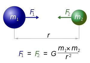
Every point mass attracts every single other point mass by a force acting along the line intersecting both points. The force is proportional to the product of the two masses and inversely proportional to the square of the distance between them.

How this simulation works

I am using software OpenGL on the CPU for all the rendering of the visuals and CPU and OpenCL for the gravity calculations. OpenCL code runs on your graphics card GPU and GPUs are great at running lots of small bits of code fast at the same time. The gravity formula maths is perfect for multi threading. Every objects velocity and acceleration can be calculated at the same time as the other objects.

The basics of using OpenCL is you fill arrays with the information you want the OpenCL code to use (for 3D gravity I am passing position, velocity, acceleration and mass of the objects), pass it to OpenCL, run the code on the GPU, and then read back the results from the GPU when it is done.

This is the current OpenCL code I am using for these latest simulations. Each of the arrays passed (posx, posy, etc) contain all the current objects, ie for a 1 million object simulation the posx array has 1,000,000 floating point values to cover every object’s X position in 3D space.

__kernel void Gravity3DKernel( __global float * posx,
		               __global float * posy
		               __global float * posz, 
		               __global float * velx, 
		               __global float * vely, 
		               __global float * velz, 
		               __global float * accx, 
		               __global float * accy, 
		               __global float * accz, 
		               __global float * mass, 
		               __global float * mingravdist)
{	
	int index=get_global_id(0);
	float dx,dy,dz,distance,force;
	float positionx=posx[index];
	float positiony=posy[index];
	float positionz=posz[index];
	float mingravdistsqr=mingravdist[index]*mingravdist[index];
	float accelerationx=0;
	float accelerationy=0;
	float accelerationz=0;
	float thismass=mass[index];
	for(int a=0; a<get_global_size(0); a++) {
		if (a!=index) {
			dx=posx[a]-positionx;
			dy=posy[a]-positiony;
			dz=posz[a]-positionz;
			distance=sqrt(dx*dx+dy*dy+dz*dz);
			dx=dx/distance;
			dy=dy/distance;
			dz=dz/distance;
			//old method - all objects are assumed to have the same mass
			//force=1/(distance*distance+mingravdistsqr);
			//new method - allows objects to have different masses
			force=(thismass*mass[a])/(distance*distance+mingravdistsqr);
			accelerationx+=dx*force;
			accelerationy+=dy*force;
			accelerationz+=dz*force;
		}
	}
	velx[index]+=accelerationx;
	vely[index]+=accelerationy;
	velz[index]+=accelerationz;
	accx[index]=accelerationx;
	accy[index]=accelerationy;
	accz[index]=accelerationz;
}

The kernel code loops through every object and calculates the forces against every other object. This is the naive unoptimized O(n2) version of the algorithm. Once all the loops are finished the new object velocity and acceleration values are read back from the GPU memory into local memory and then the CPU can access the results. All of the object positions are then updated using the new velocity and acceleration values and then displayed. For displaying the objects I am using the old software only OpenGL billboard quads. A billboard quad is a texture on a quad (rectangle) that always faces the “camera” in OpenGL. If you put a nicely shaded and transparent “blob” as the texture it looks like a simple star and blends in with other stars.

A Bug With The Shader Code

Years after I made this post it was pointed out to me by Angel in the comments that I was not comparing every object to every other object. The for loop was using get_local_size rather than get_global_size.

Once you switch to get_global_size the simulation time does increase. Also, I find the correct results are not as interesting as the incorrect ones I show in the next section. I have added a checkbox to Visions of Chaos to enable correct calculations or not. Correct uses get_global_size, incorrect uses get_local_size.

If you are trying to replicate the results from the following sample movies, change get_global_size in the for loop to get_local_size. If you want correct gravity interactions that every object is compared to every other object leave the code as is.

Results

Here is a new sample 4K resolution 3D Gravity movie.

After the last movie I went back and improved the color shading code and added the option for a “black hole”, which in this case is only a single object with a larger mass than the others. The black hole has a mass of around 100 to 500 times the other stars. Any higher and all the stars are flung out of the simulation area too quickly. Here are are some of the latest results.

The spiral galaxy like results are mostly a fluke. I started the simulation with a disk or oblate spheroid (squished sphere) of particles rotating around the origin (Y axis) with a central black hole and let it run.

After a bit more tweaking of the code and coloring algorithms the next movie was ready.

Try It Yourself

The latest 3D Gravity code is now updated and included in Visions of Chaos.

Jason.

MergeLife Cellular Automata

A new variety of cellular automata from Jeff Heaton. His original paper describing MergeLife is here, but he also made the following video that clearly explains how the rules work.

Jeff’s MergLife page also has more info and examples you can run online.

MergeLife is now included with Visions of Chaos. I haven’t added the genetic mutations yet, but you can repeatedly click the random and mutate buttons and see what new patterns emerge.

Jason.

Cellular Automata Explained – Part 1

My attempt at explaining cellular automata. Aimed at someone who has no real knowledge of how CAs work.

If you look at some online definitions of CAs you will see explanations like this and this. You can try and understand them, but probably be still left confused.

1D Cellular Automata

OK, let’s start at the simplest form of cellular automata, the one dimensional cellular automata.

A one dimensional CA consists of a line of row of cells. Each cell can be alive (on) or dead (off).

The first row of the image above is how this cellular automaton begins. It has 1 single centered alive (black) cell surrounded by dead (white) cells.

1D CA Rules

Cellular automata change states and evolve based on simple rules. The rules apply to every cell in the CA at the same time each step.

For the above image, the rules are as follows;

This shows the 8 possible rules for this CA. Each new cell state depends on itself and it’s 2 neighbors in the previous state.

The first rule (with the 3 black squares above a single white square) means that if the current cell and its two neighbors are black that cell will become a white cell the next step of the CA.

The second rule means that if a cell and its left neighbor are black but its right neighbor is white, the cell will be white in the next step.

The rest of the 6 rules are the same principal and cover all possible combinations of white and black cells.

You apply these rules to every cell in the CA each step. Here is a nice animation courtesy of Wikipedia showing how the rules are applied to a row of cells and the next step of the CA resulting from the rules.

Once the rules have been applied to all the cells, that step is completed. For 1D CA the easiest way to display them is to show each of the steps under the last in a 2D grid. The first 15 steps are shown in the grid above.

1D CA Rule Numbers

Looking again at the rule for this CA

you will notice that there are a series of 1’s and 0’s under the rules. 0 for if the rule creates a dead (white) cell and 1 if the rule creates an alive (black) cell. This series of 1’s and 0’s can be converted into a binary string that can then be converted into a number. For 8 digit binary numbers the numbers will range from 0 (for 00000000) to 255 (for 11111111).

These 1D CA’s have 256 possible combinations of rules. Rule 30 (shown above) is the conversion of 00011110 binary into digital 30. Being able to refer to each rule as a single number makes it easier to state which rule you are talking about.

More steps

If you follow the above rule repeatedly for more steps it evolves like this

From such simple rules some interesting structures arise within in. This specific rule has been used to generate random numbers (you can keep track of the center pixel going down the image and use it to create random numbers). You can see more info about Rule 30 here.

So what about the other 255 1D CA rules?

You can see the results of all 256 rules here.

An interesting result is rule 22.

Rule 22 results in a structure of triangles within triangles. This is a famous fractal pattern called the Sierpinski Triangle and it tends to pop up all over the place in cellular automata and fractals.

The End – for now

Hopefully by now you have a basic understanding of cellular automata. The main points to know are;

1. CAs are based on a grid of cells that are alive or dead.
2. The CA runs/updates/steps by running a set of rules on all the cells at the same time.
3. The same rules are then applied to the new cells and the process repeats itself.

The one dimensional cellular automata are kind of bland and once you seen the possible 256 rules there isn’t much excitement, but understanding 1D first makes the transition into higher dimensions and more complex rules easier to grasp.

If you want to experiment with these 1D CAs yourself, you can download Visions of Chaos. Open the 1D CA mode dialog and suddenly the options should be more clear to you now.

There is even an option that takes the CA steps and maps them into music. You can also print a catalog of all the 256 rules with more details.

If any of the above is not clear, please comment and let me know.

Jason.

Mandelbrot Foam

A new variation on Mandelbrot Fractals.

The Mandelbrot Foam formula was from this forum post.

Shaders to create these fractals are now included in the Custom Formula Editor mode of Visions of Chaos.

Jason.