Line based 3D Strange Attractors

Posted by softologyblog on January 21, 2018

History

I have played with 3D strange attractors in the past (see here and here). Those attractors were formed by plotting millions of points in 3D space.

The points plotted will seem to jump around randomly at first, but after a few million or so points they do start to form the attractor shapes.

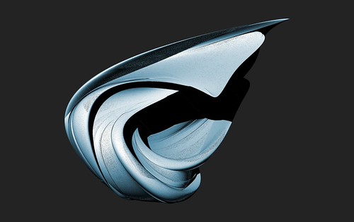
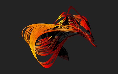
The attractors in this post are slightly different. The attractor formula is still iterated in the same way, but in these attractors the points form a series of points along a curve. This curve can be plotted as a line in 3D space. I couldn’t find an official term difference between the attractors plotted by points vs the attractors plotted by lines. If there is one, let me know.

Inspiration

My journey into these attractors started by first seeing this web GLSL based plotter created by Mikael Hvidtfeldt Christensen.

Mikael was inspired by these awesome renderings by Chaotic Atmospheres.

Mikael also points to the home page of Jürgen Meier that contains a long list of attractor types and source code to create them.

I had to have a go at adding these to Visions of Chaos as a new mode, so off I went.

The attractor formulas involved are fairly simple and the source code for each type really helped me get the attractor math going quickly. In the end I implemented 60 of the attractors on Jürgen’s page.

Displaying the attractors

If you use one of the attractor formulas you will end up with a long list of points in 3D space that need to be displayed.

I used a series of OpenGL cylinders between the points. This is OK but really doesn’t work as you have breaks where the cylinders do not join each other correctly. I need to implement some code to extrude a circle or other shapes along a curve when I get some time, but unless you look very closely at the following movie you won’t notice the breaks.

Red and blue glasses anaglyph display

I have also added a 3D Strange Attractors album to my flickr gallery. If you have a pair of the old anaglyph red and blue glasses you can also see some anaglyph images of the attractors in this gallery.

Here is a movie of the anaglyph attractors rotating.

Cross-eyed stereogram

Another method of seeing these in 3D. Slightly cross your eyes until the 2 images merge into 1.

You may need to find that sweet spot between movie size and your distance from the screen to see the 3D at its best.

Some quick programmer tips

If you work from Jürgen Meier’s excellent reference you may (or at least I did) notice some of the attractors do not plot the same as his. The cause of this is most likely (other than a typo in parameters) will be the delta value. The delta is that “small amount” that each iteration of the attractor is multiplied by to stop it “blowing up” and having all the points escape to infinity. If you notice your plot exploding lower the delta by a factor of ten and try again. Similarly some delta values seem too small so the plot takes a long time. Increasing delta will speed up the plot. You just need to tweak the delta until you get that sweet spot between accuracy and speed.

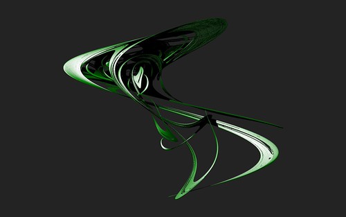
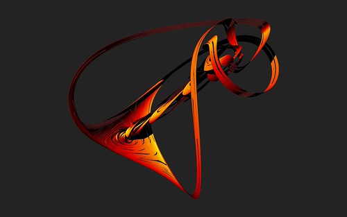
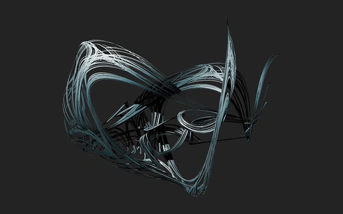
Another point to mention. When you calculate any strange attractor (this applies for 2D and 3D when using points or lines) you need to skip plotting the first thousand points. This allows the attractor to “settle” into the attractor’s basin. Otherwise you get a line or points that are not part of the attractor. An example is this image

That little squiggly tail at the bottom is where the plot started and is not part of the attractor. I have seen this same error in articles in reputable journals too sometimes, with images of strange attractors with tails that are not part of the basin of attraction.

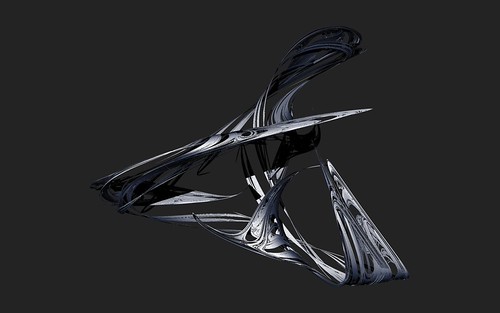
Once you have the attractor points they will all tend to fall within different XYZ coordinate ranges. Scaling them all into a fixed range (in my case I used -0.5 to +0.5) allows them all to be centered on the screen when rendering and allows them to be easily shaded by converting XZY to RGB. All it took was a bit of whiteboard scribbling and I had nicely centered attractors.

Jason.

2D Strange Attractors

Posted by softologyblog on March 4, 2017

Strange Attractors are plots of relatively simple formulas. They are created by repeating (or iterating) a formula over and over again and using the results at each iteration to plot a point. The result of each iteration is fed back into the equation. After millions of points have been plotted fractal structures appear. The repeated points fall within a basin of attraction (they are attracted to the points that make up these shapes).

I recently revisited my old strange attractor code in Visions of Chaos to add some new variations. This post will show many of the strange attractor formulas and some 4K resolution sample images they create. The images were created using over 1 billion points each. They have also been oversampled at least 3×3 pixels to reduce aliasing artifacts.

Bedhead Attractor

Discovered by Ivan Emrich.


x and y both start at 1.0

xnew=sin(x*y/b)*y+cos(a*x-y)
ynew=x+sin(y)/b

Variables a and b are floating point values bewteen -1 and +1

A=0.65343 B=0.7345345

A=-0.81 B=-0.92

A=-0.64 B=0.76

A=0.06 B=0.98

A=-0.67 B=0.83

Clifford Attractor

Discovered by Clifford A Pickover. I found them explained on Paul Bourke‘s page here.


x and y both start at 0.1

xnew=sin(a*y)+c*cos(a*x)
ynew=sin(b*x)+d*cos(b*y)

Variables a,b,c and d are floating point values bewteen -3 and +3

A=-1.7 B=1.3 C=-0.1 D=-1.21

A=-1.7 B=1.8 C=-0.9 D=-0.4

A=1.5 B=-1.8 C=1.6 D=2

A=-2.239 B=-2.956 C=1.272 D=1.419

A=-1.7 B=1.8 C=-1.9 D=-0.4

Fractal Dream Attractor

Discovered by Clifford A Pickover and discussed in his book “Chaos In Wonderland”.


x and y both start at 0.1

xnew=sin(y*b)+c*sin(x*b)
ynew=sin(x*a)+d*sin(y*a)

Variables a and b are floating point values bewteen -3 and +3
Variables c and d are floating point values between -0.5 and +1.5

A=-0.966918 B=2.879879 C=0.765145 D=0.744728

A=-2.9585 B=-2.2965 C=-2.8829 D=-0.1622

A=-2.8276 B=1.2813 C=1.9655 D=0.597

A=-1.1554 B=-2.3419 C=-1.9799 D=2.1828

A=-1.9956 B=-1.4528 C=-2.6206 D=0.8517

Gumowski-Mira Attractor

The Gumowski-Mira equation was developed in 1980 at CERN by I. Gumowski and C. Mira to calculate the trajectories of sub-atomic particles. It can also be used to create attractor images.


x and y both start at any floating point value between -20 and +20

t=x
xnew=b*y+w
w=a*x+(1-a)*2*x*x/(1+x*x)
ynew=w-t

The a and b parameters can be any floating point value between -1 and +1.

Initial X=0 Initial Y=0.5 A=0.008 B=-0.7

Initial X=-0.723135391715914 Initial Y=-0.327585775405169 A=0.79253300698474 B=0.345703079365194

Initial X=-0.312847771216184 Initial Y=-0.710899183526635 A=0.579161538276821 B=-0.820410779677331

Initial X=-0.325819793157279 Initial Y=0.48573582014069 A=0.062683217227459 B=-0.436713613104075

Initial X=0.78662442881614 Initial Y=0.919355855789036 A=0.900278024375439 B=0.661233567167073

Hopalong Attractor

The Hopalong attractor was discovered by Barry Martin.


x and y both start at 0

xnew=y-1-sqrt(abs(b*x-1-c))*sign(x-1)
ynew=a-x-1

The parameters a, b and c can be any floating point value between 0 and +10.

A=7.16878197155893 B=8.43659746693447 C=2.55983412731439

A=7.7867514709942 B=0.132189802825451 C=8.14610984409228

A=9.74546888144687 B=1.56320227775723 C=7.86818214459345

A=9.8724800767377 B=8.66862616268918 C=8.66950439289212

A=9.7671244922094 B=4.10973468795419 C=3.78332691499963

Jason Rampe 1

A variation I discovered while trying random formula changes.


x and y both start at 0.1

xnew=cos(y*b)+c*sin(x*b)
ynew=cos(x*a)+d*sin(y*a)

Variables a, b, c and d are floating point values between -3 and +3

A=2.6 B=-2.5995 C=-2.9007 D=0.3565

A=1.8285 B=-1.8539 C=0.3816 D=1.9765

A=2.5425 B=2.8358 C=-0.8721 D=2.7044

A=-1.8669 B=1.2768 C=-2.9296 D=-0.4121

A=-2.7918 B=2.1196 C=1.0284 D=0.1384

Jason Rampe 2

Another variation I discovered while trying random formula changes.


x and y both start at 0.1

xnew=cos(y*b)+c*cos(x*b)
ynew=cos(x*a)+d*cos(y*a)

Variables a, b, c and d are floating point values between -3 and +3

A=1.546 B=1.929 C=1.09 D=1.41

A=2.907 B=-1.9472 C=1.2833 D=1.3206

A=0.8875 B=0.7821 C=-2.3262 D=1.5379

A=-2.4121 B=-1.0028 C=-2.2386 D=0.274

A=-2.9581 B=0.927 C=2.7842 D=0.6267

Jason Rampe 3

Yet another variation I discovered while trying random formula changes.


x and y both start at 0.1

xnew=sin(y*b)+c*cos(x*b)
ynew=cos(x*a)+d*sin(y*a)

Variables a, b, c and d are floating point values between -3 and +3

A=2.0246 B=-1.323 C=-2.8151 D=0.2277

A=1.4662 B=-2.3632 C=-0.4167 D=2.4162

A=-2.7564 B=-1.8234 C=2.8514 D=-0.8745

A=-2.218 B=1.4318 C=-0.3346 D=2.4993

A=1.2418 B=-2.4174 C=-0.7112 D=-1.9802

Johnny Svensson Attractor

See here.


x and y both start at 0.1

xnew=d*sin(x*a)-sin(y*b)
ynew=c*cos(x*a)+cos(y*b)

Variables a, b, c and d are floating point values between -3 and +3

A=1.40 B=1.56 C=1.40 D=-6.56

A=-2.538 B=1.362 C=1.315 D=0.513

A=1.913 B=2.796 C=1.468 D=1.01

A=-2.337 B=-2.337 C=0.533 D=1.378

A=-2.722 B=2.574 C=1.284 D=1.043

Peter DeJong Attractor

See here.


x and y both start at 0.1

xnew=sin(y*a)-cos(x*b)
ynew=sin(x*c)-cos(y*d)

Variables a, b, c and d are floating point values between -3 and +3

A=0.970 B=-1.899 C=1.381 D=-1.506

A=1.4 B=-2.3 C=2.4 D=-2.1

A=2.01 B=-2.53 C=1.61 D=-0.33

A=-2.7 B=-0.09 C=-0.86 D=-2.2

A=-0.827 B=-1.637 C=1.659 D=-0.943

A=-2 B=-2 C=-1.2 D=2

A=-0.709 B=1.638 C=0.452 D=1.740

Symmetric Icon Attractor

These attractors came from the book “Symmetry in Chaos” by Michael Field and Martin Golubitsky. They give symmetric results to the attractors formed.


x and y both start at 0.01

zzbar=sqr(x)+sqr(y)
p=alpha*zzbar+lambda
zreal=x
zimag=y
for i=1 to degree-2 do
begin
     za=zreal*x-zimag*y
     zb=zimag*x+zreal*y
     zreal=za
     zimag=zb
end
zn=x*zreal-y*zimag
p=p+beta*zn
xnew=p*x+gamma*zreal-omega*y
ynew=p*y-gamma*zimag+omega*x
x=xnew
y=ynew

The Lambda, Alpha, Beta, Gamma, Omega and Degree parameters can be changed to create new plot shapes.

These sample images all come from paramters in the “Symmetry in Chaos” book.

L=-2.5 A=5 B=-1.9 G=1 O=0.188 D=5

L=1.56 A=-1 B=0.1 G=-0.82 O=0.12 D=3

L=-1.806 A=1.806 B=0 G=1 O=0 D=5

L=-2.195 A=10 B=-12 G=1 O=0 D=3

L=2.5 A=-2.5 B=0 G=0.9 O=0 D=3

L=-2.05 A=3 B=-16.79 G=1 O=0 D=9

L=-2.7 A=5 B=1.5 G=1.0 O=0 D=6

L=2.409 A=-2.5 B=0 G=0.9 O=0 D=23

L=-2.08 A=1 B=-0.1 G=0.167 O=0 D=7

L=-2.32 A=2.32 B=0 G=0.75 O=0 D=5

L=2.6 A=-2 B=0 G=-0.5 O=0 D=5

L=-2.34 A=2 B=0.2 G=0.1 O=0 D=5

L=-1.86 A=2 B=0 G=1 O=0.1 D=4

L=1.56 A=-1 B=0.1 G=-0.82 O=0 D=3

L=1.5 A=-1 B=0.1 G=-0.805 O=0 D=3

L=1.455 A=-1 B=0.03 G=-0.8 O=0 D=3

L=2.39 A=-2.5 B=-0.1 G=0.9 O=-0.15 D=16

3D Alternatives

Strange Attractors can also be extended into three dimensions. See here and here for my previous experiments with 3D Strange Attractors.

All of the images in this post were created using Visions of Chaos.

Jason.

Further adventures with 3D Strange Attractors

Posted by softologyblog on February 20, 2011

After the original new 3D Strange Attractor formulas I found here I have been playing with alternate formulas and came up with these 5 new types.

Here are the formulas used and some sample images of each type. The a3da[] values are parameters between -1 and +1 that control the shapes.

Rampe 6
xnew=z*sin(a3da[0]*x)-cos(a3da[1]*y)
ynew=x*sin(a3da[2]*y)+cos(a3da[3]*z)
znew=y*sin(a3da[4]*z)-cos(a3da[5]*x)

Rampe 7
xnew=z*sin(a3da[0]*x)-cos(a3da[1]*y)
ynew=x*cos(a3da[2]*y)+sin(a3da[3]*z)
znew=y*sin(a3da[4]*z)-cos(a3da[5]*x)

Rampe 8
xnew=z*sin(a3da[0]*x)-cos(y)
ynew=x*cos(a3da[1]*y)+sin(z)
znew=y*sin(a3da[2]*z)-cos(x)

Rampe 9
xnew=y*sin(a3da[0]*x)-arccos(a3da[1]*y)+sin(a3da[2]*z)
ynew=z*sin(a3da[3]*x)-arccos(a3da[4]*y)+sin(a3da[5]*z)
znew=x*sin(a3da[6]*x)-arccos(a3da[7]*y)+sin(a3da[8]*z)

Rampe 10
xnew=y*sin(a3da[0]*x)-cos(a3da[1]*y)+arcsin(a3da[2]*z)
ynew=z*sin(a3da[3]*x)-cos(a3da[4]*y)+sin(a3da[5]*z)
znew=x*sin(a3da[6]*x)-cos(a3da[7]*y)+sin(a3da[8]*z)

All of the above formulas are now implemented in the latest version of Visions Of Chaos.

I have more ideas to expand new attractor formuals in future versions of Visions Of Chaos. Firstly is to get a decent formula compiler implented so the user can try formulas easily by typing in the 3 formulas for xnew, ynew and znew. Once that works the next obvious evolution is to get it to genetically evolve and mutate the formulas like I have done for Genetic Art in the past.

Jason.

3D Strange Attractors

Posted by softologyblog on October 19, 2009

After some experimenting, I came up with the following 5 new formulas for generating 3D strange attractors. They all use SIN and COS like Cliff Pickover did when he was creating strange attractors.

All of these formulas were found by trial and error of changing and trying new formulas. In the future it would be interesting to use a genetic/evolutionary system of randomizing formulas and trying to find interesting results automatically.

The x,y and z variables are intialized to 0. Newx, newy and newz are temporary variables to hold the new x,y and z values until the new point is calculated. The parameters in italics a to i are floating point values in the range of -1 to +1 that alter/control the resulting image.

These sample images contain up to one billion plotted points to smooth them out. Each pixel is an average of a super sampled 3×3 grid to help remove aliasing (this is similar to rendering the image at 9 times the size and then downsizing it in an image processing application). The first two samples of each formula are rendered using a z-buffer technique to give them a solid appearance. The third sample of each formula is rendered using an accumulation buffer that shades the pixels based on the number of times each pixel is hit which allows you to see the internal structure of the attractor.

Rampe1 Attractor
newx=z*sin(a*x)+cos(b*y)
newy=x*sin(c*y)+cos(d*z)
newz=y*sin(e*z)+cos(f*x)

rampe1_01