Visions of Chaos has supported flames for years now, but something I recently revisited was detecting interesting looking flame fractals.
The flame fractals appearance are controlled by the coefficients, probabilities, transformations and multiplier values (the lower table floating point values in the above dialog), but 99% of the time if you just set random values it will lead to boring images. Boring here means an image that is just a few straight lines, a circle, or only a few pixels.
Searching for an interesting flame fractal means repeatedly randomizing the controlling parameters and testing the resulting plotted points. Here is a snippet of code I use to test each random set of parameters.
     xp:=0.05;
     yp:=0.05;
     //skip first 1000 iterations to allow it to settle down
     for loop:=1 to 1000 do iterate_point;

     repeat
           thisxp:=xp;
           thisyp:=yp;

           //iterate the next point
           iterate_point;

           //test if tending to a point
           if (abs(thisxp-xp)<1e-10) and (abs(thisyp-yp)<1e-10) then
           begin
                TestFlameParameters:=false;
                exit;
           end;

           //check if unbounded, ie values are getting too large
           if (abs(xp)>10000) or (abs(yp)>10000) then
           begin
                TestFlameParameters:=false;
                exit;
           end;

           //check for NAN
           if (isnan(xp)) or (isnan(yp)) then
           begin
                TestFlameParameters:=false;
                exit;
           end;

           //check for INF
           if (isinfinite(xp)) or (isinfinite(yp)) then
           begin
                TestFlameParameters:=false;
                exit;
           end;

           //count pixels that fall within the image area
           if (xp<xmax) then
           if (xp>xmin) then
           if (yp<ymax) then
           if (yp>ymin) then
           begin
                xplot:=trunc((xp-xmin)/abs(xmin-xmax)*width);
                yplot:=trunc((yp-ymin)/abs(ymin-ymax)*height);
                hitpixelscount[xplot,yplot]:=hitpixelscount[xplot,yplot]+1;
           end;

           inc(pointcount);

     until (pointcount=250000);

     //count pixels hit
     hits:=0;
     for y:=0 to height-1 do
         for x:=0 to width-1 do
             if hitpixelscount[x,y]>5 then inc(hits);
     if hits<trunc(width*1.5+height*1.5) then
     begin
          TestFlameParameters:=false;
          exit;
     end;
     //if it got to here then the tests all passed
The tests included in the code and the ones I found most useful are;
1. Detect tending to a single point. A lot of flames result in the iterations being attracted to a single point/pixel.
2. Unbounded. Points continue to grow outwards to infinity.
3. NAN and INF. If the floating point math returns a NAN or INF.
4. Count pixels hit. If the resulting image has too few pixels the flame picture will be boring. Counting the pixels helps detect and avoid these flames.
Using those 4 checks will skip hundreds (at least in my case) of parameters that fail one or more of the above tests. The result is when looking for new random flame fractals you skip the boring point-like and line-like displays.
The following screen shot of the flame mutator in Visions of Chaos shows a series of flames that all passed the tests. They may not all be interesting aesthetically, but there are no minimal results with just a small number of pixels.
Daniel Shiffman has been making YouTube movies for some time now. His videos focus on programming and include coding challenges in which he writes code for a target idea from scratch. If you are a coder I recommend Dan’s videos for entertainment and inspiration.
His latest live stream focused on Fractal Spirographs.
If you prefer to watch a shorter edited version, here it is.
Fractal Spirographs (aka Fractal Routlette) are generated by tracking a series (or chain) of circles rotating around each other as shown in the above gif animation. You track the chain of 10 or so circles and plot the path the final smallest circle takes. Changing the number of circles, the size ratio between circles, the speed of angle change, and the constant “k” changes the resulting plots and images.
How I Coded It
As I watched Daniel’s video I coded my own version. For my code (Delphi/pascal) I used a dynamic array of records to hold the details of each circle/orbit. This seemed the simplest approach to me for keeping track of a list of the linked circles.
type orbit=record
     x,y:double;
     radius:double;
     angle:double;
     speed:double;
end;
Before the main loop you fill the array;
//parent orbit
orbits[0].x:=destimage.width/2;
orbits[0].y:=min(destimage.width,destimage.height)/2;
orbits[0].radius:=orbits[0].y/2.5;
orbits[0].angle:=0;
orbits[0].speed:=0;
rsum:=orbits[0].radius;
//children orbits
for loop:=1 to numorbits-1 do
begin
     newr:=orbits[loop-1].radius/orbitsizeratio;
     newx:=orbits[loop-1].x+orbits[loop-1].radius+newr;
     newy:=orbits[loop-1].y;
     orbits[loop].x:=newx;
     orbits[loop].y:=newy;
     orbits[loop].radius:=newr;
     orbits[loop].angle:=orbits[loop-1].angle;
     orbits[loop].speed:=power(k,loop-1)/sqr(k*k);
end;
Then inside the main loop, you update the orbits;
//update orbits
for loop:=1 to numorbits-1 do
begin
     orbits[loop].angle:=orbits[loop].angle+orbits[loop].speed;
     rsum:=orbits[loop-1].radius+orbits[loop].radius;
     orbits[loop].x:=orbits[loop-1].x+rsum*cos(orbits[loop].angle*pi/180);
     orbits[loop].y:=orbits[loop-1].y+rsum*sin(orbits[loop].angle*pi/180);
end;
and then you use the last orbit positions to plot the line, ie
Once the code was working I rendered the following images and movie. They are all 4K resolution to see the details. Click the images to see them full size.
Here is a 4K movie showing how these curves are built up.
Fractal Spirographs are now included with the latest version of Visions of Chaos.
Finally, here is an 8K Fulldome 8192×8192 pixel resolution image. Must be seen full size to see the fine detailed plot line.
To Do
Experiment with more changes in the circle sizes. The original blog post links to another 4 posts here, here, here and here and even this sumo wrestler
Plenty of inspiration for future enhancements.
I have already experimented with 3D Spirographs in the past, but they are using spheres rotating within other spheres. Plotting the sqheres rotating around the outside of other spheres should give more new unique results.
The other day I saw this YouTube video of a Belousov-Zhabotinsky Cellular Automaton (BZ CA) by John BitSavage
After a while of running in an oscillating state it begins to grow cell like structures. I had never seen this in BZ CAs before. I have seen similar cell like growths in Digital Inkblot CAs and in the Yin Yang Fire CA. Seeing John’s results different to the usual BZ CA was what got me back into researching BZ in more depth.
The Belousov-Zhabotinsky Reaction
Belousov-Zhabotinsky Reactions (see here for more info) are examples of a chemical reactions that can oscillate between two different states and form intetesting patterns when performed in shallow petri dishes.
Here are some sample high res images of real BZ reaction by Stephen Morris. Click for full size.
and some other images from around the Internet
and some sample movies I found on YouTube
The Hodgepodge Machine Cellular Automaton
Back in August 1988, Scientific American‘s Computer Recreations section had an article by A. K. Dewdney named “The hodgepodge machine makes waves”. After a fair bit of hunting around I could not find any copies of the article online so I ended up paying $8 USD to get the issue in PDF format. The PDF is a high quality version of the issue, but $8 is still a rip off.
In the article Dewdney describes the “hodgepodge machine” cellular automaton designed by Martin Gerhardt and Heike Schuster of the University of Bielefeld in West Germany. A copy of their original paper can be seen here.
How the Hodgepodge Machine works
The inidividual cells/pixels in the hodgepodge automaton have n+1 states (between 0 and n). Cells at state 0 are considered “healthy” and cells at the maximum state n are said to be “ill”. All cells with states inbetween 0 and n are “infected” with the larger the state representing the greater level of infection.
Each cycle of the cellular automaton a series of rules are applied to each cell depending on its state.
(a) If the cell is healthy (i.e., in state 0) then its new state is [a/k1] + [b/k2], where a is the number of infected cells among its eight neighbors, b is the number of ill cells among its neighbors, and k1 and k2 are constants. Here “[]” means the integer part of the number enclosed, so that, for example, [7/3] = [2+1/3] = 2.
(b) If the cell is ill (i.e., in state n) then it miraculously becomes healthy (i.e., its state becomes 0).
(c) If the cell is infected (i.e., in a state other than 0 and n) then its new state is [s/(a+b+1)] + g, where a and b are as above, s is the sum of the states of the cell and of its neighbors and g is a constant.
The parameters given for these CA are usual q (for max states), k1 and k2 (the above constants) and g (which is a constant for how quickly the infection tends to spread).
My previous limited history experimenting with BZ
Years ago I implemented BZ CA in Visions of Chaos (I have now correctly renamed the mode Hodgepodge Machine) and got the following result. This resolution used to be considered the norm for YouTube and looked OK on lower resolution screens. How times have changed.
The above run used these parameters
q=200
k1=3
k2=3
g=28
Replicating Gerhardt and Miner’s results
Gerhadt and Miner used fixed values of k1=2 and k2=3. The majority of their experiments used a grid size of q=20 (ie only 20×20 cells) without a wraparound toroidal world. This leaves the single infection spreading g variable to play with. Their paper states they used values of g between 1 and 10, but I get no spirals with g in that range.
Here are a few samples which are 512×512 sized grids with wraparound edges and many thousands of generations to be sure they had finally settled down. Each cell is 2×2 pixels in size so they are 1024×1024 images.
q=100, k1=2, k2=3, g=5
q=100, k1=2, k2=3, g=20
q=100, k1=2, k2=3, g=25
q=100, k1=2, k2=3, g=30
Results from other parameters
q=100, k1=3, k2=3, g=10
q=100, k1=3, k2=3, g=15
q=100, k1=3, k2=3, g=20
Extending into 3D
The next logical step was extending it into three dimensions. This blog post from Rudy Rucker shows a 3D BZ CA from Harry Fu back in 2004 for his Master’s degree writing project. I must be a nerd as I whipped up my 3D version over two afternoons. Surprisingly there are no other references to experiments with 3D Hodgepodge that I can find.
The algorithms are almost identical to their 2D counterparts. The Moore neighborhood is extended into three dimensions (so 26 neighbors rather than 8 in the 2D version). It is difficult to see the internal structures as they are hidden from view. Methods I have used to try and see more of the internals are to slice out 1/8th of the cubes and to render only some of the states.
Clicking these sample images will show them in 4K resolution.
q=100, k1=1, k2=18, g=43 (150x150x150 grid)
q=100, k1=1, k2=18, g=43 (150x150x150 grid – same as previous with a 1/8th slice out to see the same patterns are extending through the 3D structure)
q=100, k1=1, k2=18, g=43 (150x150x150 grid – same rules again, but this time with only state 0 to state 50 cells being shown)
q=100, k1=2, k2=3, g=15 (150x150x150 grid)
q=100, k1=3, k2=6, g=31 (150x150x150 grid)
q=100, k1=4, k2=6, g=10 (150x150x150 grid)
q=100, k1=4, k2=6, g=10 (150x150x150 grid – same rules as the previous image – without the 1/8th slice – with only states 70 to 100 visible)
Download Visions of Chaos if you would like to experiment with both 2D and 3D Hodgepodge Machine cellular automata. If you find any interesting rules please let know in the comments or via email.
In the video game industry older games get remastered all the time. Hardware power improves so older games are adapted to have better graphics and sound etc. So for a nostalgic trip into history (at least for me) it was time for some Visions of Chaos movie remasters.
After recently adding the new Custom Formula Editor into Visions of Chaos I decided to go back and re-render some sample Mandelbrot movies at 4K 60fps. Most of these Mandelbrot movie scripts go back to the earliest days of Visions of Chaos even before I first released it on the Internet. The only changes made have been to add more sub frames so they render more smoothly and last longer.
Thanks to the new formula editor using OpenGL shading language and a recent NVidia GPU all the movie parts rendered overnight. Every frame was 2×2 supsampled so the equivalent of rendering an image 4 times as large and then downsampling to increase the quality. The original movie was a 46 GB XVID encoded AVI before YouTube put it through all of its internal recoding steps.
DLA is a simple process to simulate in the computer and was one of my first simulations that I ever coded. For the simplest example we can consider a 2D scenario that follows the following rules;
1. Take a grid of pixels and clear all pixels to white.
2. Make the center pixel black.
3. Pick a random edge point on any of the 4 edges.
4. Create a particle at that edge point.
5. Move the particle randomly 1 pixel in any of the 8 directions (N,S,E,W,NE,NW,SE,SW). This is the “diffusion”.
6. If the particle goes off the screen kill it and go to step 4 to create a new particle.
7. If the particle moves next to the center pixel it gets stuck to it and stays there. This is the “aggregation”. A new particle is then started.
Repeat this process as long as necessary (usually until the DLA structure grows enough to touch the edge of the screen).
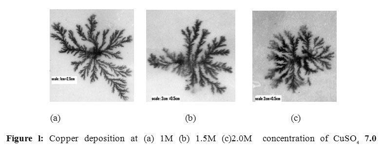
When I asked some of my “non-nerd” aquaintances what pattern would result from this they all said a random blob like pattern. In reality though the pattern produced is far from a blob and more of a coral like branched dendritic structure. When you think about it for a minute it does make perfect sense. Because the moving particles are all coming from outside the fixed structure they have less of a chance of randomly walking between branches and getting to the inner parts of the DLA structure.
All of the following sample images can be clicked to see them at full 4K resolution.
Here is an image created by using the steps listed above. Starting from a single centered black pixel, random moving pixels are launched from the edge of the screen and randomly move around until they either stick to the existing structure or move off the screen.
Start configuration: Single centered black pixel
Random pixels launched from: rectangle surrounding existing structure
Neighbours checked for an existing pixel: N, S, E, W, NE, NW, SE, SW
Particles stick condition: when they move next to a single stuck particle
The change in this next example is that neighbouring pixels are only checked in the N, S, E and W directions. This leads to horizonal and vertical shaped branching.
Start configuration: Single centered black pixel
Random pixels launched from: rectangle surrounding existing structure
Neighbours checked for an existing pixel: N, S, E, W
Particles stick condition: when they move next to a single stuck particle
There are many alternate ways to tweak the rules when the DLA simulation is running.
Paul Bourke’s DLA page introduces a “stickiness” probability. For this you select a probability of a particle sticking to the existing DLA structure when it touches it.
Decreasing probability of a particle sticking leads to more clumpy or hairy structures.
Start configuration: Single centered black pixel
Random pixels launched from: rectangle surrounding existing structure
Neighbours checked for an existing pixel: N, S, E, W, NE, NW, SE, SW
Particles stick condition: 0.5 chance of sticking when they move next to a single stuck particle
Start configuration: Single centered black pixel
Random pixels launched from: rectangle surrounding existing structure
Neighbours checked for an existing pixel: N, S, E, W, NE, NW, SE, SW
Particles stick condition: 0.1 chance of sticking when they move next to a single stuck particle
Start configuration: Single centered black pixel
Random pixels launched from: rectangle surrounding existing structure
Neighbours checked for an existing pixel: N, S, E, W, NE, NW, SE, SW
Particles stick condition: 0.01 chance of sticking when they move next to a single stuck particle
Another method is to have a set count of hits before a particle sticks. This gives similar results to using a probability.
Start configuration: Single centered black pixel
Random pixels launched from: rectangle surrounding existing structure
Neighbours checked for an existing pixel: N, S, E, W, NE, NW, SE, SW
Particles stick condition: once a moving particle has hit stuck particles 15 times
Start configuration: Single centered black pixel
Random pixels launched from: rectangle surrounding existing structure
Neighbours checked for an existing pixel: N, S, E, W, NE, NW, SE, SW
Particles stick condition: once a moving particle has hit stuck particles 30 times
Start configuration: Single centered black pixel
Random pixels launched from: rectangle surrounding existing structure
Neighbours checked for an existing pixel: N, S, E, W, NE, NW, SE, SW
Particles stick condition: once a moving particle has hit stuck particles 100 times
Start configuration: Single centered black pixel
Random pixels launched from: rectangle surrounding existing structure
Neighbours checked for an existing pixel: N, S, E, W, NE, NW, SE, SW
Particles stick condition: once a moving particle has hit stuck particles 1000 times
Another change to experiment with is having a threshold neighbour count random particles have to have before sticking. For example in this next image all 8 neighbours were checked and only 1 hit was required to stick, but the moving particles needed to have at least 2 fixed neighbour particles before they stuck to the existing structure.
The first 50 hits only need 1 neighbour. This build a small starting structure which all the following hits stick to with 2 or more neighbours.
Start configuration: Single centered black pixel
Random pixels launched from: rectangle surrounding existing structure
Neighbours checked for an existing pixel: N, S, E, W, NE, NW, SE, SW
Particles stick condition: once a moving particle has 2 or more stuck neighbours
That gives a more clumpy effect without the extra “hairyness” of just adding more hit counts before sticking.
Start configuration: Single centered black pixel
Random pixels launched from: rectangle surrounding existing structure
Neighbours checked for an existing pixel: N, S, E, W, NE, NW, SE, SW
Particles stick condition: once a moving particle has 3 or more stuck neighbours
This seems a happy balance to get thick branches yet not too fuzzy ones.
Start configuration: Single centered black pixel
Random pixels launched from: rectangle surrounding existing structure
Neighbours checked for an existing pixel: N, S, E, W, NE, NW, SE, SW
Particles stick condition: once a moving particle has 3 or more stuck neighbours and has hit 3 times
The next two examples launch particles from the middle of the screen with the screen edges set as stationary particles.
Start configuration: Edges of screen set to black pixels
Random pixels launched from: middle of the screen
Neighbours checked for an existing pixel: N, S, E, W, NE, NW, SE, SW
Particles stick condition: once a moving particle has 1 or more stuck neighbours
Start configuration: Edges of screen set to black pixels
Random pixels launched from: middle of the screen
Neighbours checked for an existing pixel: N, S, E, W, NE, NW, SE, SW
Particles stick condition: once a moving particle has 3 or more stuck neighbours
These next three use a circle as the target area. Particles are launched from the center of the screen.
Start configuration: Circle of black pixels
Random pixels launched from: middle of the screen
Neighbours checked for an existing pixel: N, S, E, W, NE, NW, SE, SW
Particles stick condition: once a moving particle has 1 or more stuck neighbours
Start configuration: Circle of black pixels
Random pixels launched from: middle of the screen
Neighbours checked for an existing pixel: N, S, E, W, NE, NW, SE, SW
Particles stick condition: once a moving particle has 2 or more stuck neighbours
Start configuration: Circle of black pixels
Random pixels launched from: middle of the screen
Neighbours checked for an existing pixel: N, S, E, W, NE, NW, SE, SW
Particles stick condition: once a moving particle has 3 or more stuck neighbours
This next image is a vertical 2D DLA. Particles drop from the top of the screen and attach to existing seed particles along the bottom of the screen. Color of sticking particles uses the color of the particle they stick to.
Start configuration: Bottom of screen is fixed particles
Random pixels launched from: top of the screen
Neighbours checked for an existing pixel: S, SE, SW
Particles stick condition: once a moving particle has 1 or more stuck neighbours
Dendron Diffusion-limited Aggregation
Another DLA method is Golan Levin’s Dendron DLA. He kindly provided java source code so I could experiment with Dendron myself. Here are a few sample images.
Hopefully all of the above examples shows the wide variety of 2D DLA possible and the various methods that can produce them. This post was mainly going to be about 3D DLA, but I got carried away trying all the 2D possibilities above.
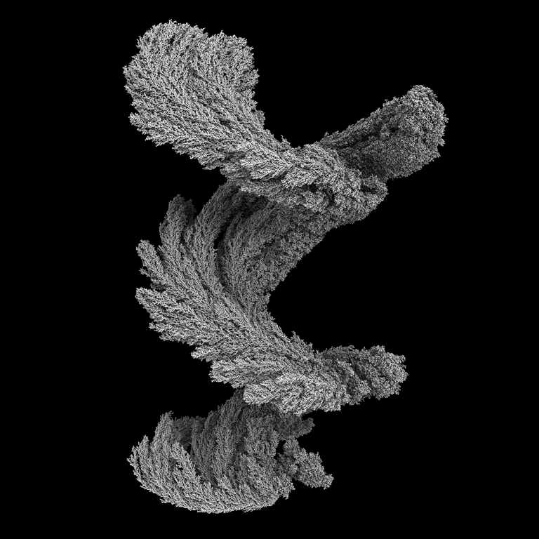
3D Diffusion-limited Aggregation
DLA can be extended into 3 dimensions. Launch the random particles from a sphere rather than a surroundiong circle. Check for a hit against the 27 possible neighbours for each 3D grid cell.
For these movies I used default software based OpenGL spheres. Nothing fancy. Slow, but still managable with some overnight renders.
In this first sample movie particles stuck once they had 6 neighbours. In the end their are approximately 4 million total spheres making up the DLA structure.
This second example needed 25 hits before a particle stuck and a particle needed 5 neighbours to be considered stuck. This results in a much more dense coral like structure.
Note: see here for my latest much improved 3D DLA results.
A Quick Note About Ambient Occlusion
Ambient occlusion is when areas inside nooks and crannies are shaded darker because light would have more trouble reaching them. Normally to get accurate ambient occlusion you raytrace a hemisphere of rays from the surface point seeing how many objects the rays intersect. The more hits, the darker the shading. This is a slow process. For the previous 3D DLA movies I cheated and used a method of counting how many neighbour particles the current sphere has. The more neighbours the darker the sphere was shaded. This gives a good enough fake AO.
Programming Tip
A speedup some people do not realise is when launching random particles. Use a circle or rectangle just slightly larger than the current DLA structure. No need to start random points far from the structure.
Other Diffusion-limited Aggregation Links
For many years now the ultimate inspiration in DLA for me has been Andy Lomas.
Another change Andy uses is to launch the random walker particles in patterns that influence the structure shape as in this next image.
Future Changes
1. More particles. The above 2 movies have between 4 and 5 million particle spheres at the end of the movies. Even more particles would give more natural looking structures like the Andy Lomas examples.
2. Better rendering. Using software (non-GPU) OpenGL works but it is slow. Getting a real ray traced result supporting real ambient occlusion and global illumination would be more impressive.
3. Controlled launching of particles to create different structure shapes other than a growing sphere.
Mobile phones and tablets have had nice high DPI displays for a long time now. PC screens have started to catch up and 4K monitors are starting to come down in price and will become the standard in the future.
The good thing about higher DPI screens is that there are many more pixels on the same sized screen so text and images are shown much more clearly.
The bad thing is most applications (especially older programs) are not aware of High DPI scaling settings. If an application does not support scaling Windows just “zooms” the application window to a larger size. This leads to blurry text that most people complain about. So you either set the scaling factor to 100% which leads to tiny text or you live with blurry text.
Over the past few weeks I have been working on making Visions of Chaos high DPI aware. The end result is that it will now run happily on all scale settings and higher 4K monitors without the text being too tiny to read or blown up and blurry. The menus and all text within Visions of Chaos will scale according to your Windows settings and remain smooth and crisp to read.
High DPI in Visions of Chaos
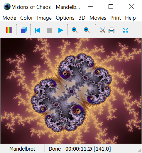
Prior to Visions of Chaos being DPI aware Windows would just scale the output window like in a photo editor app. The following shows how the Visions of Chaos window looks at 150% scaling under Windows 10 on a 4K display.
This leads to the blurred text and the generated image (set to 480×360 pixels in size) is shown onscreen also stretched and blurred to 725 pixels wide.
Here is the same window using the latest version of Visions of Chaos that is DPI aware. The text fonts are scaled to a larger size so they remain crisp and smooth. The fractal image that has been set to 480×360 pixels is exactly 480×360 monitor pixels.
Windows is still playing catch up with higher resolution DPI support, but it will hopefully get better as 4K monitors become the standard. At least you can be confident that Visions of Chaos will continue to be usable and readable at high DPI settings.
Now I can get back to adding new features to Visions of Chaos.
This is a quick post showing an alternative way to display the result of plotting double, triple and quadruple pendulums.
Based on my previous magnetic pendulum simulation and plots I had the idea to try a similar plot style for the double, triple and quadruple pendulums.
If you simulate a pendulum attached to another pendulum in zero gravity without any friction you get a system that runs continuously and creates a plot like the following gif animation.
With 3 pendulums the plot is more complex.
With 4 it is even more complex.
Another way to visualize this is to plot a 2D image with the X axis being 0 to 360 degrees of the first pendulum and the Y axis being 0 to 360 degrees of the second pendulum. The simulations are run for 5000 steps at each pixel location. Depending on which quadrant of the screen the pendulum is in after the 5000 steps determines the color of the pixel (red, green, blue or yellow). The top left pixel sets the pendulum angles to both 0, runs the simulation for 5000 steps and because the end of the two pendulums is located in the lower left quarter of the screen the pixel is colored green. This process is then repeated for the remaining pixels of the image.
Here is the result for the double pendulum
and the triple
and the quadruple
The original code was taking 12 minutes for a 320×240 image using the simplest double pendulum code. I am patient, but not that patient. A quick recode into GLSL and the GPU took over the number crunching and now it is rendering 640×480 results in under 2 seconds.
Here is a gif animation of the double pendulum plot with the number of simulation iterations increasing each frame.
If you are interested in seeing the GLSL shader source code click here.
The above plotting and shader code is now included with Visions Of Chaos if you just want to experiment without having to do any coding.
Here are the simple steps to generate Langton’s Ant.
1. Start with a blank 2D grid of white cells/pixels.
2. Place a virtual ant in the middle cell.
3. If the ant is on a white cell it turns the pixel black, turns 90 degrees right and then moves one cell forward.
4. If the ant is on a black cell it turns the pixel white, turns 90 degrees left and then moves one cell forward.
5. Step 3 and 4 are repeated for as long as required.
Here is a nice GIF file courtesy of Wikipedia that shows how the first 200 steps of Langton’s Ant evolve.
At first the ant travels around in a roughly blob shaped random pattern, but after a while (around 10,000 steps) the ant starts to build a structured pathway as in the following GIF animation.
Structures like that are referred to as highways. The above highway would continue to grow forever on a large enough grid.
Rule strings for a wider variety of Ants
Langton’s Ant can be represented by the rule “RL” which is the direction the ant turns depending on the underlying cell color. R for a black cell and L for a blue cell (as in the above animation).
An extension to Langton’s Ant is to allow more than 2 characters. For example, if you try RRLL as a rule it gives the following cardioid like structure over time (click for a larger detailed image).
With more characters in the rule string you use more colors. In the above cardioid example the first R character is black and then the other 3 colors are shaded between a light and dark blue.
A simple way of referring to the different rules is to use a rule number. To get a rule number, you follow these steps;
1. Convert the rule string into a binary string. RRLL -> 1100.
2. Convert that binary string into a decimal number. 1100 = 12.
Here are some other examples with their rule numbers showing the variety of patterns that can emerge from these very simple rules. Click on each of the images to see the higher resolution originals.
Rule 9
Rule 262 – Diagonal scaffolding like structures
Rule 908 – Builds a rougher jagged highway
Rule 1080 – Spiral
Rule 8383 – Build Sierpinski Triangle patterns as it grows
The next logical step was to extend into 3D space. I was trying to work out how to handle and program an ant turning in 3 dimensions when I came across Dr Heiko Hamann‘s page on 3D Langton’s Ants. He generously provides some source code here that has the required matrix manipulation required to get the ant turning in 3D space. Have a look if you are interested in implementing your own 3D version of Langton’s Ant.
Once I got the code working I ran a brute force search over the first 20,000 rule numbers. It is harder to see structures within the blobs of random that tend to emerge, but a few interesting results did occur. One thing you get is a lot of very basic highways, so the same emergence of highways in 2D does carry over to 3D.
Here are a few examples I found so far and their corresponding rule numbers. Click to see the larger original images.
Rule 318 – An example of one of the many highways
Rule 1042 – Creates more cubic structures and then builds a vertical highway
Rule 4514 – Slowly builds a complex vertical highway
Rule 6046 – Builds a vertical sprouting highway from a virtual seed
Rule 6738 – Corkscrew highway
Rule 9513 – Zigzag highway
Rule 10952 – After a long time building a seemingly random blob it starts generating a triangle shaped highway
Rule 17416 – Generates plate like interlocking 3D puzzle pieces and then a complex highway
OBJ Export
Visions Of Chaos also supports exporting the 3D Ant Automata to OBJ files. Here are some examples of 3D Ants exported to OBJ files and imported into and rendered in Blender. I really am a total amateur with Blender but these images show some potential with nice ambient occlusion.
Experiment with Ant Automata
If you want to see any of these automata being built or want to experiment with other rules, download Visions Of Chaos.
If you find any new interesting rules let me know.
If you are a nerd then you most likely have heard of Karl Sims. If you haven’t heard of him give his page a browse as there is some good stuff there.
I have admired and respected him since his work in Genetic Images back in 1993 that inspired all three of my attempts at Genetic Art so far. I still have a few more ideas on new Genetic Art methods to experiment with and share when I get some spare time.
I noticed his latest work as I was browsing Reaction Diffusion videos on YouTube.
Check these two RD samples Karl put up on YouTube.
The most impressive aspect of those is the shading that gives them the 3D look. (Aussies can confirm the almost exact reflectance of the second example to Vegemite). Remember that the output of these Reaction Diffusion equations is strictly 2D. The bulging 3D look is based on calculating the slope between neighbouring pixels. Or at least that is how I do it in Visions Of Chaos, but Karl’s versions seem so much more 3Dish than mine. See his images here that are awesome.
As always he inspires me (and I am sure many others) to do better.
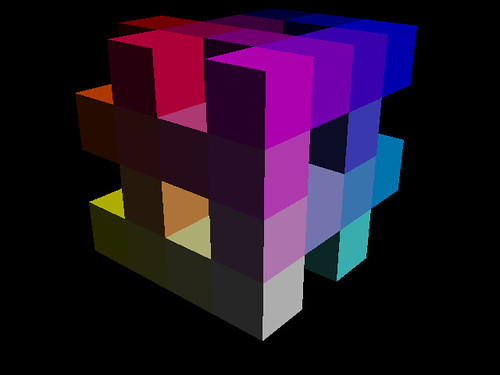
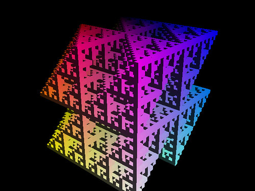
Take a regular cube. It can be broken up into eight smaller cubes. Remove one or more of those eight cubes. Repeat the removal process for each of the remaining smaller cubes. Repeat again as many times as you like.
This gives you 256 possible unique fractal cube structures. So you take a “rule number”, convert it to a binary string and then use the bninary string to determine which of the eight subcubes are removed.
Here is an example of rule number 132 after 2, 3, 4 and 5 iterations.
and here is a movie of the level 5 rule 132 fractal rotating.
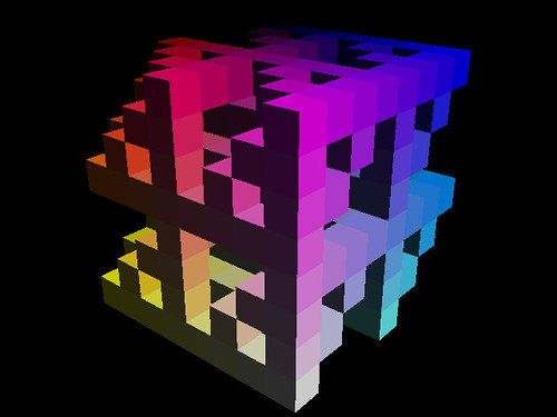
You can also apply the same principal, but based on random numbers. Each set of subcubes has a 1 in 8 chance of being removed. The rule number then becomes the pseudo random number generator seed value.
Here is an example movie of random rule 1155 rotating.
I have included these new fractal cubes in the latest version of Visions Of Chaos.