This post has been in a draft state for at least a couple of years now. I revisit it whenever I get inspiration for a new idea. I wasn’t going to bother posting it until I had a better solution to the problem, but maybe these ideas can trigger a working solution in someone else’s mind.
Compared to my other blog posts this one is more rambling as it follows the paths I have gone down so far when trying to solve this problem.
Objective
Cellular automata tend to have huge parameter search spaces to find interesting results within. The vast majority of rules within this space will be junk rules with only a small fraction of a percentage being interesting rules. I have spent way too many hours repeatedly trying random rules when looking for new interesting cellular automata. Between the boring rules that either die out or rules that go chaotic there is that sweet spot of interesting rules. Finding these interesting rules is the problem.
My ideal goal has always been to be able to run random rules repeatedly hands free and have software that is “clever” enough to determine the difference of interesting vs boring results. If the algorithms are good enough at detecting interesting then you can come back to the computer hours or days later and have a set of rules in a folder with preview images and/or movies to check out.
I want the smarts to be smart enough to work with a variety of CA types beyond the basic 2 state 2D cellular automata. Visions of Chaos contains many varieties of cellular automata with varying maximum cell states, dimensions and neighborhoods that I ultimately would like to be able to click a “Look for interesting rules” button.
Interesting Defined
Interesting is a very loose term. Maybe a few examples will help define what I mean when I say interesting.
Boring results are when a CA stabilizes to a fixed pattern or a pattern with very minimal change between steps.
Chaotic results are when the CA turns into a screen of static with no real discernible patterns or features like gliders or other CA related structures. For a CA classifier these rules are also boring.
Interesting is anything else. Rules like Game of Life, Brian’s Brain and others that create evolvable structures that survive after multiple cycles of the CA. This is what I want the software to be able to detect.
My Previous Search Methods
1. Random rules. Repeatedly generate random rules hoping to see an interesting result. Tedious to say the least, although the majority of the interesting cellular automata rules I have found over the years have been through repeatedly trying different random rules. While a boring TV show or movie is on I can repeatedly hit F3, F4 and Enter in Visions of Chaos while looking for interesting results. F3 stops the current CA running, F4 shows the settings dialog, Enter clicks the Random Rule button.
2. Brute force all possible rules. Only applicable for when the total number of rules is small (possible for some of the simpler 1D CAs). Most 2D CAs have millions or billions of possible rules and brute force rendering them all and then checking manually is impossible.
3. Mutating existing interesting rules. If you get an interesting rule, you can try mutating the rule slightly to try alternatives that may behave similarly yet better to the rule. Slightly usually means toggling one of the survival/birth checkboxes on/off. This has occasionally helped me find interesting rules or refine a rule to that sweet spot. The problem with CAs is that even changing one checkbox will usually result in a completely different result. The good results do not tend to “clump” together in the parameter space.
The rest of this blog post contains methods others and myself have tried to classify cellular automata behavior.
Wolfram Classification
Stephen Wolfram defined a rough set of 4 classifications for CAs.
Class 1: Nearly all initial patterns evolve quickly into a stable, homogeneous state. Any randomness in the initial pattern disappears.
Class 2: Nearly all initial patterns evolve quickly into stable or oscillating structures. Some of the randomness in the initial pattern may filter out, but some remains. Local changes to the initial pattern tend to remain local.
Class 3: Nearly all initial patterns evolve in a pseudo-random or chaotic manner. Any stable structures that appear are quickly destroyed by the surrounding noise. Local changes to the initial pattern tend to spread indefinitely.
Class 4: Nearly all initial patterns evolve into structures that interact in complex and interesting ways, with the formation of local structures that are able to survive for long periods of time.
Classes 1 to 3 would be considered “boring” for anyone trying random rules. Class 4 is that “sweet spot” of CAs that something interesting happens between dying out and chaotic explosions.
You can look at a CA after it has been discovered and put it into one of those 4 categories but that doesn’t help detecting interesting rules in Class 4.
Other Methods From Various Papers
Here are some other classification methods in papers I found or saw mentioned elsewhere. The mathematics is beyond me for most of them. I wish papers included a small snippet of source code with them that shows the math. I always find it much easier understanding and implementing some source code rather than try and understand formal equations.
Behavioral Metrics
Search Of Complex Binary Cellular Automata_Using_Behavioral_Metrics.
Entropy
Wolfram’s Universality And Complexity In Cellular Automata discusses “entropy” values that I don’t understand.
Wuensche’s Classifying Cellular Automata Automatically
Lyapunov Exponents
Stability Of Cellular Automata Trajectories Revisited : Branching Walks And Lyapunov Profiles.
Towards The Full Lyapunov Sprectrum Of Elementary Cellular Automata.
Kolmogorov–Chaitin Complexity
Asymptotic Behaviour And Ratios Of Complexity In Cellular Automata.
Genetic Algorithms
Searching For Complex CA Rules With GAs.
Evolving Continuous Cellular Automata For Aesthetic Objectives.
Extracting Cellular Automaton Rules Directly From Experimental Data.
Other Papers
Pattern Generation Using Likelihood Inference For Cellular Automata. 1D CAs.
MergeLife
Jeff Heaton uses genetic mutations to evolve cellular automata.
Langton’s Lambda
Chris Langton defined a single number that can help predict if a CA will fall within the ordered realm. See his paper Computation at the edge of chaos for the mathematical definitions etc.
Langton called this number lambda. According to this page Lambda is calculated by counting the number of cells that have just been “born” that step of the CA and dividing it by the total CA cells. This gives a value between 0 and 1.
L = newlyborn/totalcellcount
L within 0.01 and 0.15 means a good rule to further investigate.
So if the grid is 20×20 in size and there were 50 cells that were newly born that CA cycle, then lambda would be 50/20×20=0.125
I skip the first 100 CA cycles to allow the CA to settle down and then average the lambda value for the next 50 steps.
As stated here there is no single value of lambda that will always give an interesting result. Langton’s paper and example applet are only concerned with 1D CA examples. I really want to find methods to search and classify 2D, 3D (and even 4D) cellular automata.
Rampe’s Lambdas
For lack of a better name, these are the “Rampe’s Lambda” values I experimented with as alternatives to Langton’s Lambda.
R1 = newlyborn/newlydead
R1 within 0.9 and 1.1 means a good rule to further investigate.
R2 = abs(newlyborn-newlydead)/totalcellcount
R2 within 0.001 and 0.005 means a good rule to further investigate.
R3 = (newlyborn+newlydead)/totalcellcount
R3 within 0.01 and 0.8 means a good rule to further investigate.
R4 = ((newlyborn/totalcellcount)+(newlydead/totalcellcount))/2
R4 within 0.01 and 0.23 means a good rule to further investigate.
R5 = % change in Langton’s Lambda between the last and current CA cycle
R5 within 0.01 and 0.1 means a good rule to further investigate.
Again, skip the first 100 cycles of the CA and then use the average lambda from the following 50 cycles.
Lambda Results
All of them (both Langton and my “Rampe” variations) are next to useless from my tests. I ran a bunch of known good rules and got mixed results. All the lambda’s gave enough false positives to not be of any use in searching for interesting new rules. You may as well use a random number generator to classify the rules.
Maybe they can be used to weed out the extreme class 1, 2 and 3 uninteresting dead rules, but they are not useful for classifying if a class 4 like result is interesting or not.
Fractal Dimension
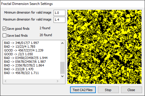
Another method I tried is finding the fractal dimension of the CA image using box counting. Fractal dimensions are unlike the usual 1D, 2D and 3D fixed dimensions and for a 2D image are and floating point value between 0 and 2.
The above screenshot shows the fractal dimension tests on existing sample interesting CA files. The results are all over the place with no “sweet spot” of dimension correlating to interesting. The way it works is that each CA is run for 50 steps, the image is converted to black and white (non black pixels in the image are changed to white) and then the dimension is calculated using the box counting method.
Increasing the range of dimension for “good” detection may result in the known interesting rules to pass the tests, but it then thinks a lot of uninteresting rules are then interesting, meaning you still need to manually sort good vs bad.
A fractal dimension between 1.0 and 1.4-1.5 can help weed out obvious “bad” results, but is really not helpful in hands free searching.
Compression Based Searching
Another new interesting idea on CA searching comes from Hugo Cisneros, Josef Sivic and Tomas Mikolov. Using data compression algorithms to rate CAs.
Their paper “Evolving Structures in Complex Systems” available here is an interesting read.
Source code accompanying the paper is provided here.
Neural Networks – Part 1
This was an idea I had for a while. Train a neural network to detect if a CA rule is interesting or not.
I was able to implement a rudimentary neural network system after watching these excellent videos from Dan Shiffman.
I went from almost zero knowledge of the internals of neural networks to much more comfortable and being able to code a working NN system. If you want to learn about the basics of coding a neural network I highly recommend Dan’s playlist.
For a neural network to be able to give you meaningful output (in this case if a CA rule is interesting or not) it needs to be trained with known good and bad data.
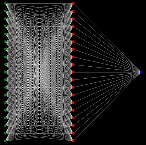
I tried creating a neural network with 19 inputs (9 for survival states, 9 for birth states and 1 for number of states) to cover the possible CA settings, ie
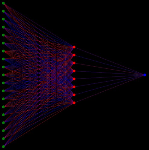
The neural network has 19 inputs, a number of neurons in the hidden layer and a single output neuron that does the interestingness prediction.
I mainly kept the hidden neuron count the same as the inputs, but I did experiment with other counts as the next diagram shows.
The known good and bad rules are fed through the neural network in random order for 10 million or more times. You can see how well the network is “learning” by tracking the mean squared error. As you repeatedly feed the network known data the error value should drop meaning the network is becoming more accurate at predicting the results you train it with.
Once the network is trained, you can run random rules and see if the prediction of the network matches your rating of if the CA is interesting or not. You can also repeatedly try random rules until they pass a threshold level of interesting. Every time a prediction is made the human can rate if the detection was correct. These human ratings are added back to the good and bad rule training pool so they can be used the next time the network is trained.
The end result is “just OK”. I used a well trained network (with a mean squared error of around 0.001) and got it to repeatedly try random rules until it found a rule it predicted would be interesting. The results are not always interesting. More interesting than purely sitting there clicking random repeatedly as I have done in the past, but there are still a lot of not interesting rules spat out. If I let the network run for a few hours and got it to save every rule it predicted to be interesting I would still have a tedious process of weeding out the actual interesting rules.
I don’t think inputs from survival and birth rules is the best way of doing this. This is because a toggle of a single survival or birth checkbox will usually drastically change the results from interesting to boring or just chaos. Also changing the maximum states each cell can have by 1 will cause well behaved rules to change into chaotic mess results.
One idea I need to try is using a basic NN like this that uses the lambda values above for inputs. Maybe then it can work out which combination of lambdas (and maybe fractal dimension) work together to create good rules. This is worth experimenting with when I get some time.
Neural Networks – Part 2
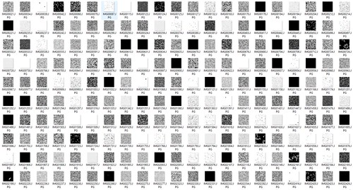
This time I am trying to get the network to detect interesting CAs by using images from a frame of the CAs. For each of the known good and bad rules I take the 100th frame as an input. I also repeat each of the rules 100 times to get 100 samples of each rule.
If I use a 64×64 sized grayscale image then there will now be 4,096 inputs to the network. Add another 100 hidden nodes and that makes a large and much slower network when training.
Run the CA rules on a 64×64 sized grid, convert the image pixels into the 4,096 inputs and train the network.
So far, no good results. The mean squared error falls very slowly. Maybe it would get better after days of training, but I am not that patient yet.
This online example and this article show how this method (a fully connected neural network) is never as accurate as a convolutional neural network. So, onto Part 3…
Neural Networks – Part 3
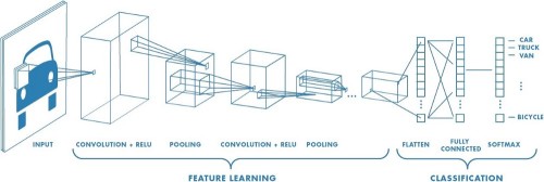
My next idea was to try using Convolutional Neural Networks. See here for a nice explanation of convolutional neural networks.
CNN’s are made for image processing, feature extraction and detection. If a CNN can be trained to recognize digits and tell if a photo is of a cat or a dog then I should be able to use a CNN to “look at” a frame of a cellular automaton and tell me if it is interesting or not.
After watching a bunch of YouTube university lectures and tutorials on CNNs I decided not to extend my existing neural network code to handle CNNs. For the network sizes I will be training I need a real world library. I chose Google’s TensorFlow.
TensorFlow supports GPU acceleration with CUDA and is magnitudes faster and more reliable than anything I could code.
Once I managed to get Python, TensorFlow, Keras, CUDA and cuDNN installed correctly I was able to execute Python scripts from within Visions of Chaos and successfully run the example TensorFlow CNN MNIST code. That showed I had all the various components working as expected.
Creating Training Data for the CNN
Acquiring clean and accurate training data is vital for a good model. The more data the better.
I used the following steps to create a lot of training images;
1. Take a bunch of CA rules that I had previously ranked as either good or bad.
2. Run all of them over a 128×128 sized grid for 100 steps and save the 100th frame as a grayscale jpg file.
3. Step 2 can be repeated multiple times to increase the amount of training data. CAs starting from a random grid will always give you a unique 100th frame so this is an easy way to generate lots more training data.
4. Copy some of the generated images into a test folder. I usually move 1/10th of the total generated images into a test folder. These will be used to evaluate how accurate the model is at predictions once it has been trained. You want test data that is different to the data used to train and validate the model.
Quantity and Dimensions of Training Data Images
I tried image sizes between 32×32 pixels and 128×128 pixels. I also tried various zoomed in CA images with each cell being 2×2 pixels rather than a single pixel per cell.
For image counts I tried between 10,000 up to 300,000.
After days of generating images and training and testing models I found a good balance between image size and model accuracy was images 128×128 pixels in size with a single pixel per CA cell (so a CA grid of 128×128 too).
I also experimented with blurring the images thinking that may help search for more general patterns, but it did not seem to make any difference in the number found or accuracy of results.
One thing working with neural networks teaches you is patience. Generating the images is the slowest part of these experiments. If anyone is willing to gift me some decent high end CPUs and GPUs I would put them to good use.
Custom Input for CNNs
The best videos I found on using CNNs with custom images were these videos on YouTube by sentdex. Parts 1 to 6 of that playlist got me up and running.
Creating the Training Data for TensorFlow
Once you have your training images they need to be converted into a data format that TensorFlow can be trained with.
Again, I recommend the following sentdex video that covers how to create the training data.
The process to convert the training images into training data is fast and should not take longer than a minute or two.
Model Variations
Time to actually use this training data to train a convolutional neural network (what TensorFlow calls a model).
There are a wide variety of model and layer types to experiment with. For CNNs you basically start with one or more Conv2D layers followed by one or more Dense layers and finally a single output node to predict a probability of the image being good or bad.
Here are some models I tried during testing. From various sources and videos and pages I have seen. Running on an Nvidia 1080 GPU took around 2 hours per model to train (50 epochs each with 100,000 training images), which seemed lightning fast after waiting 30 hours for my training images to generate.
# Version 1# Original model from sentdex videos# https://youtu.be/WvoLTXIjBYUmodel = Sequential()model.add(Conv2D(64, (3,3), input_shape = X.shape[1:]))model.add(Activation("relu"))model.add(MaxPooling2D(pool_size=(2,2)))model.add(Conv2D(64, (3,3)))model.add(Activation("relu"))model.add(MaxPooling2D(pool_size=(2,2)))model.add(Flatten())model.add(Dense(64))model.add(Activation("relu"))model.add(Dense(1))model.add(Activation("sigmoid"))model.compile(loss="binary_crossentropy",optimizer="adam",metrics=["accuracy"])model.fit(X, y, batch_size=50, epochs=50, validation_split=0.3)
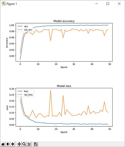
When the 50 epochs finish, you can plot the accuracy and loss vs the validation accuracy and loss.
Version 1 gave these results;
test loss, test acc: [0.13674676911142003, 0.9789666691422463]
98% accuracy with a loss of 13%
When I test a different unique set of images as test data I get;
14500 good images predicted as good – 301 good images predicted as bad – 97.97% predicted correctly
14653 bad images predicted as bad – 184 bad images predicted as good – 98.76% predicted correctly
One thing the above “Model loss” graph shows is overfitting. The val_loss graph should follow the loss graph and continue to go down. Instead of going down the line starts going up around the 5th epoch. This is an obvious sign of overfitting. Overfitting is bad. We don’t want overfitting. See here for more info on overfitting and how to avoid it.
The second suggestion from here mentions dropouts. Dropouts remove random links between nodes in the model network as it trains. This can help reduce overfitting. So let’s give that a go.
# Version 2# Original model from sentdex videos# https://youtu.be/WvoLTXIjBYU# Adding dropouts to stop overfittingmodel = Sequential()model.add(Conv2D(64, (3,3), input_shape = X.shape[1:]))model.add(Activation("relu"))model.add(MaxPooling2D(pool_size=(2,2)))model.add(Dropout(0.4))model.add(Conv2D(64, (3,3)))model.add(Activation("relu"))model.add(MaxPooling2D(pool_size=(2,2)))model.add(Dropout(0.4))model.add(Flatten())model.add(Dense(64))model.add(Activation("relu"))model.add(Dropout(0.4))model.add(Dense(1))model.add(Activation("sigmoid"))model.compile(loss="binary_crossentropy",optimizer="adam",metrics=["accuracy"])model.fit(X, y, batch_size=50, epochs=50, validation_split=0.3)
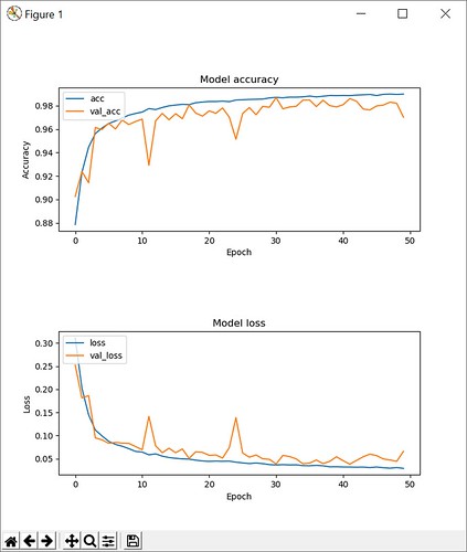
50 epochs finished with this graph.
Now the validation loss continues to generally go down with the loss graph. This shows overfitting is no longer occurring.
Version 2 gave these results;
test loss, test acc: [0.037338864829847204, 0.9866000044345856]
98% accuracy with a 13% loss
When I test a different unique set of images as test data I get;
14151 good images predicted as good – 68 good images predicted as bad – 99.52% predicted correctly
14326 bad images predicted as bad – 12 bad images predicted as good – 99.92% predicted correctly
# Version 3# https://towardsdatascience.com/applied-deep-learning-part-4-convolutional-neural-networks-584bc134c1e2model = Sequential()model.add(Conv2D(32, (3,3), input_shape = X.shape[1:]))model.add(Activation("relu"))model.add(MaxPooling2D(pool_size=(2,2)))model.add(Conv2D(64, (3,3)))model.add(Activation("relu"))model.add(MaxPooling2D(pool_size=(2,2)))model.add(Conv2D(128, (3,3)))model.add(Activation("relu"))model.add(MaxPooling2D(pool_size=(2,2)))model.add(Conv2D(128, (3,3)))model.add(Activation("relu"))model.add(MaxPooling2D(pool_size=(2,2)))model.add(Flatten())model.add(Dropout(0.5))model.add(Dense(512))model.add(Activation("relu"))model.add(Dense(1))model.add(Activation("sigmoid"))model.compile(loss="binary_crossentropy",optimizer="adam",metrics=["accuracy"])model.fit(X, y, batch_size=50, epochs=50, validation_split=0.3)
Graphs looked good without any obvious overfitting.
Version 3 gave these results;
test loss, test acc: [0.03628389219510306, 0.9891333370407422]
98% accuracy with 3% loss. Getting better.
When I test a different unique set of images as test data I get;
14669 good images predicted as good – 59 good images predicted as bad – 99.60% predicted correctly
14490 bad images predicted as bad – 62 bad images predicted as good – 99.57% predicted correctly
# Version 4# http://www.dsimb.inserm.fr/~ghouzam/personal_projects/Simpson_character_recognition.htmlmodel = Sequential()model.add(Conv2D(32, (3,3), input_shape = X.shape[1:]))model.add(Conv2D(32, (3,3)))model.add(Activation("relu"))# BatchNormalization better than Dropout? https://www.kdnuggets.com/2018/09/dropout-convolutional-networks.html# model.add(BatchNormalization())model.add(MaxPooling2D(pool_size=(2,2)))model.add(Dropout(0.25))model.add(Conv2D(64, (3,3)))model.add(Conv2D(64, (3,3)))model.add(Activation("relu"))# BatchNormalization better than Dropout? https://www.kdnuggets.com/2018/09/dropout-convolutional-networks.html# model.add(BatchNormalization())model.add(MaxPooling2D(pool_size=(2,2)))model.add(Dropout(0.25))model.add(Conv2D(128, (3,3)))model.add(Conv2D(128, (3,3)))model.add(Activation("relu"))# BatchNormalization better than Dropout? https://www.kdnuggets.com/2018/09/dropout-convolutional-networks.html# model.add(BatchNormalization())model.add(MaxPooling2D(pool_size=(2,2)))model.add(Dropout(0.5))model.add(Flatten())model.add(Dense(64))model.add(BatchNormalization())model.add(Activation("relu"))model.add(Dense(32))model.add(BatchNormalization())model.add(Activation("relu"))model.add(Dense(16))model.add(BatchNormalization())model.add(Activation("relu"))model.add(Dense(1))model.add(Activation("sigmoid"))model.compile(loss="binary_crossentropy",optimizer="adam",metrics=["accuracy"])model.fit(X, y, batch_size=50, epochs=50, validation_split=0.3)
For this model I threw in multiple ideas from all previous models and more.
Version 4 gave these results;
test loss, test acc: [0.031484683321298994, 0.9896000043551128]
99% accuracy with a 3% loss. Best result so far.
When I test a different unique set of images as test data I get;
14383 good images predicted as good – 119 good images predicted as bad – 99.18% predicted correctly
14845 bad images predicted as bad – 4 bad images predicted as good – 99.97% predicted correctly
For the rest of my tests I used Version 4 for all training.
Tweaking your CNN models
See the sentdex videos above for a good example of how to tweak models and see how the variations rate. Use TensorBoard to see how they compare and optimize them.
TensorBoard has other interesting histograms it will generate from your training like the following. I have no idea what this is telling me yet, but they look cool. Using histograms did seem to slow down the training with extended pauses between epochs, so unless you need them I recommend disabling them.
Testing the Trained Model
Now it is finally time to put the model to the test.
Randomly set a CA rule, run it for 100 generations and then use model.predict on the 100th frame. This takes around 6 seconds per random rule.
The model.predict function returns a floating point value between 0 and 1.
Between 0 and 0.2 are classified as bad.
0.2 to 0.95 are classified as unsure.
0.95 to 1 are classified as good.
The prediction accuracy is better than any of the other methods shown previously in this post.
The rules it did detect in the bad category were all bad, so it does a great job there. No interesting rules got incorrectly classified as bad from my tests. I can safely ignore rules classified as bad which speeds up the search time as I don’t have to re-run the rules and create a sample movie.
The detected good rules did have a blend of interesting and boring/chaotic, but there were a lot less of them to check. Roughly 1% of total random rules are classified as good. The rules the model incorrectly predicts as interesting can be moved into the “known bad” folder and can be added to the next trained model (another 40 hours or so of my PC churning away generating images and training a new model).
The rules it predicted in the unsure 0.2 to 0.95 range did have features that were in the range between good and bad. Some of them would have made excellent good samples if only they were not as chaotic and “busy”.
Results
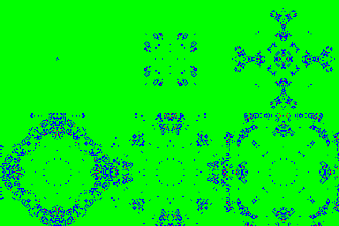
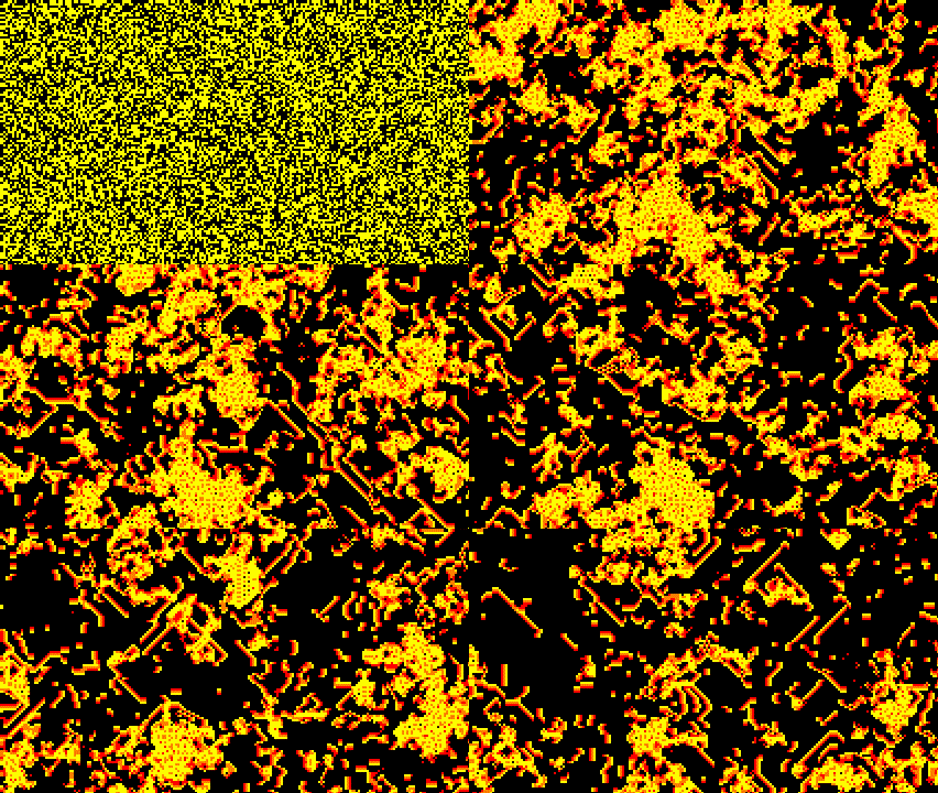
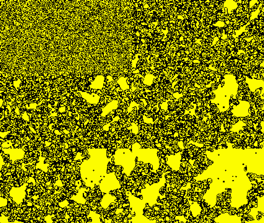
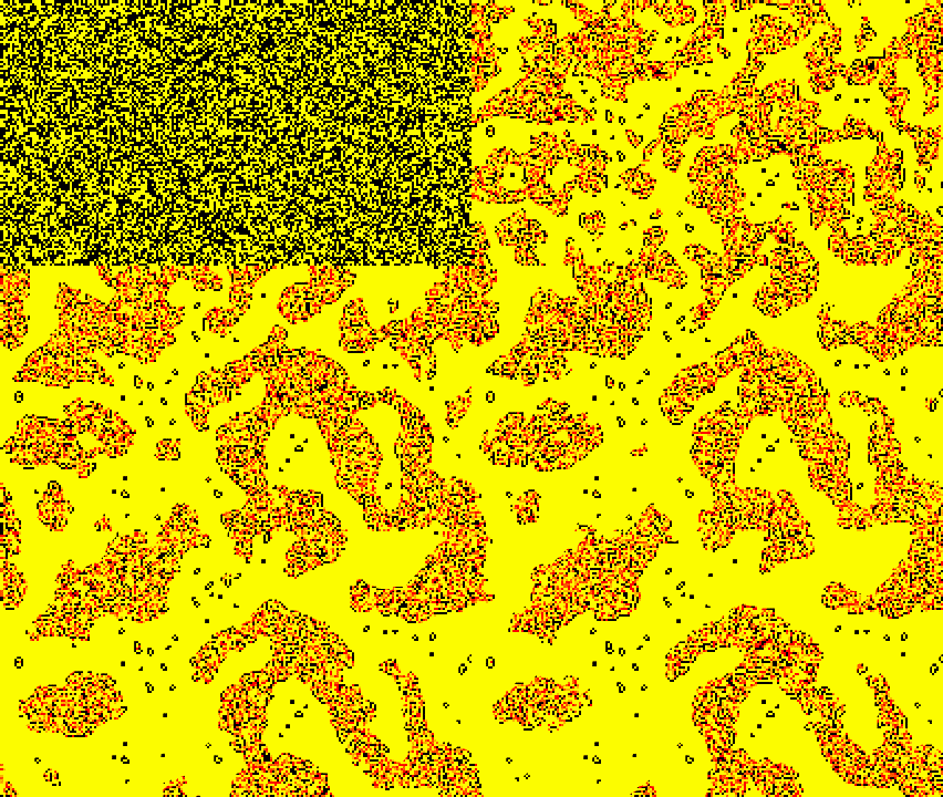
Here are some examples found from overnight convolutional neural network searches.
Other CNN Problems and Ideas
One problem is that CNNs seem to only detect shapes/gliders/patterns that are similar to the training data. After days of testing self searching with the CNN models there were no brand new different rules discovered. Just a bunch of very similar to existing rules and maybe a few slight tweaks. For example if a CNN is trained using only examples of Conway’s Game of Life CA then it is not going to predict Brian’s Brain is interesting if it randomly tries the rule for Brian’s Brain. The CNN needs to have previously seen the rule(s) it will detect as interesting. I did see slight variations found and scored as interesting, but for a new CA type without a lot of “good” rules to train on the CNN is not going to have problems finding new/different interesting rules. The main reason I want a “search for interesting” function is for when I have a new type of CA without a lot of known good rules. I want the search to be able to work without needing hundreds or thousands of examples of already rated good vs bad. Otherwise I need to sit there trying random rules for hours and manually rate them good or bad before training a new model specific to that CA rule.
Maybe using single frames is not the best idea. Maybe the difference between the 99th and 100th frame? Maybe a blur or average of 3 frames? This is still to be experimented with when I have another week to spend generating images and training and testing new models.
Then I thought maybe I am over training the models. If you train a neural network for too long it will overfit and then only be able to recognize the data you trained it with. This is as if it memorizes only the good data you gave it as good. It cannot generalize to detect other different good results as good. This results in new interesting CAs being potentially classified as bad. I did try lowering the training epochs from 50 to 10 to see if that helped detect more generalized interesting CA rules but it didn’t seem to make any difference. Even lowering it to 5 epochs trained a model that was still accurate at predictions. Plus the difference between random frames of good CAs shows it can detect gliders at different locations within frames.
Rather than train a model for each type of CA, train a model with examples from multiple CA types. Try and make the model more capable of general CA detection. Maybe it could then detect newer shapes/gliders in different new CA rules if it has a good general idea of what interesting CA features are from multiple different CAs. This may work? Another one for the to do list.
Convolutional Neural Networks (and neural networks in general) are not an instant win solution. You do need to do a lot of research about the various settings and do a lot of testing to get a good model which you can then use to predict the “things” you want the model to predict. But once you get a well trained model CNNs can be almost magical in how they can learn and be useful when solving problems.
The more I experiment with and learn about neural networks only makes me want to continue the journey. They really are fascinating. Using TensorFlow and Keras are a great way to get into the world of neural networks without having to code your own neural network system from scratch. I do recommend at least coding a basic feed forward neural network to get a good grip on the basics. When you jump into Keras the terminology will make more sense. YouTube has lots of good neural network related videos.
Availability to End Users
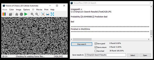
I have now included the trained (20 epochs Version 4 to hopefully leave a little room for finding more unique results) TensorFlow CNN model with Visions of Chaos. That means the end user does not need to do any image generation or training before using the CNN for searching. Python and TensorFlow need to be installed first, but after that the user can start a hands free search for interesting rules. When TensorFlow is installed and detected a search button appears on the 2D Cellular Automata dialog. Clicking Search starts a hands free random search and classification.
The other search methods above are still hidden as they do not predict interesting with a high enough accuracy.
The End (for now)
If you managed to get this far, thanks for reading.
If you have some knowledge about any of the above methods that I missed please leave a reply or get in touch and let me know.
Any other ideas for cellular automata searching and classification are also welcome.
I will continue to update this post with any other methods I find in the future.
Jason.














Heya! I’m quite interested in this idea and seriously considering messing around with this. I sort of wonder if maybe using some pre-trained convolution networks (for example the image classification stuff) could bring any improvement to this. Can also contribute with some images from random CAs to make things more fun, as I agree that throwing multiple CA`s into same model could lead to better results (maybe with some accuracy loss, but a more robust model in the end, as one would expect it would lead to higher variablity and handle cold start better). I also wonder if evaluating model performance on an out of sample holdout (for example, some CA that was not used for training the model) could lead to a better model selection.
CNNs do give the best search results so far and they are very capable of detecting patterns like gliders etc once trained.
I do need to experiment with training on images from multiple CA types. Many of the new CA methods I come up with or experiment with have very few examples of interesting rules. So to train a CNN to detect interesting the human needs to sit there for a few hours and manually rate good vs bad results that are then used to train the model.
A more general detection CNN is the ideal goal. Even if it does sacrifice some accuracy in detection. Then any time a new CA idea comes up I could let the detector run overnight and see what it finds in the morning. I have spent way too long repeatedly clicking a random button when trying new CA types in the past.
Jason.
Yep, that sounds like a very good plan 🙂
Sorry for multiple comments, just had another idea. Convolutional NN are pretty good to detect patterns, so maybe that could be used to improve the search algorithm. The idea would be to measure the similarity between patterns (something like style transfer does), to discard parameters that are stylistically similar to some existing (either train or found previously) parameters.
This is a very interesting idea that I also had in the past (but I don’t have the necessary programming skills to produce it).
A different yet related idea I had was to try and define natural selection in terms of the simulated world, so that the computer could search for simple rules which create something akin to biology.
Pingback: [Перевод] Композитор с долгой кратковременной памятью | Терещенко. Просто. Профессионально
Another possible approach: predictability. This is akin to compressibility, conceptually.
If a NN (or any other kind of predictor) can accurately predict the next frame from the previous two frames then it’s probably not interesting… the more “surprised” the NN is, the better.
This would work best with a feedback loop; each interesting new CA variant that is discovered is automatically fed back in as training data, so that similar variants can be recognized in the future.
The tricky part would be in deciding how to measure the “accuracy” of a prediction… you would want to avoid favoring chaotic results (which are unpredictable in an uninteresting way) and I’m not sure how best to do that.
I think one of the best methods that has been found so far, is looking for a high variance in the entropy of the states occurring during the time evolution of the CA.
I think it was Wuensche who wrote a paper about it
Thanks for the pointer. I added a link to Wuensche’s paper in the post. It only seems to refer to detecting 1D CAs.
Jason.